Quantum computing

The idea underlying quantum computing is that there appears to be much more information contained in a system’s quantum state than is available in the classical description of that system. So perhaps there is some way to utilize that quantum information to compute something much more efficiently than would be possible with the usual classical information.

Of course in the end, we are only able to perceive classical information. So while any useful quantum computation may bring to bear the full range of quantum information, it must render its answer in a way that we can perceive as a classical state.

In this section, we will explore how we can visualize the processing of quantum information using the examples developed so far involving wave packets and micromeasurements, all based on a particles moving in one spatial dimension. As always, we will avoid invoking the quantum measurement postulate. In the place of the traditional view of probabilistic measurement outcomes, we will see how the evolution of the wave function leads to well-separated components of the wave function, each of which corresponds to a different perceived outcome.

Quantum information

But first, classical information

First, let’s visualize the way that information is represented in a normal, classical computer. In pretty much any electronic device, information is stored as a string of bits. These bits are typically represented as zeros and ones. Physically, a bit usually corresponds to some state of electrons doing one thing vs. another. For example, a bit might be stored on a hard drive as a small magnet in which the electron spins are oriented one way or the other, or on a solid state drive as more or fewer electrons trapped within an element of the device. When information is being processed, a bit is usually represented as the presence or absence of an electrical voltage in a wire. But in the abstract, we can just think of the bits as a string of \(N\) zeros and ones, such as “00110010” if \(N=8\).

A neat and tidy way to visualize the state of a set of bits is shown in Fig. QC.1. The two possible states of a single bit can be viewed as two dots along a line. The state of that bit at any given time can be indicated by filling in one of the dots. If we flip that bit, we can swap which bit is filled in.

Figure QC.1

Visualization of a system of one, two, and three classical bits. The yellow dot indicates the state of the system.

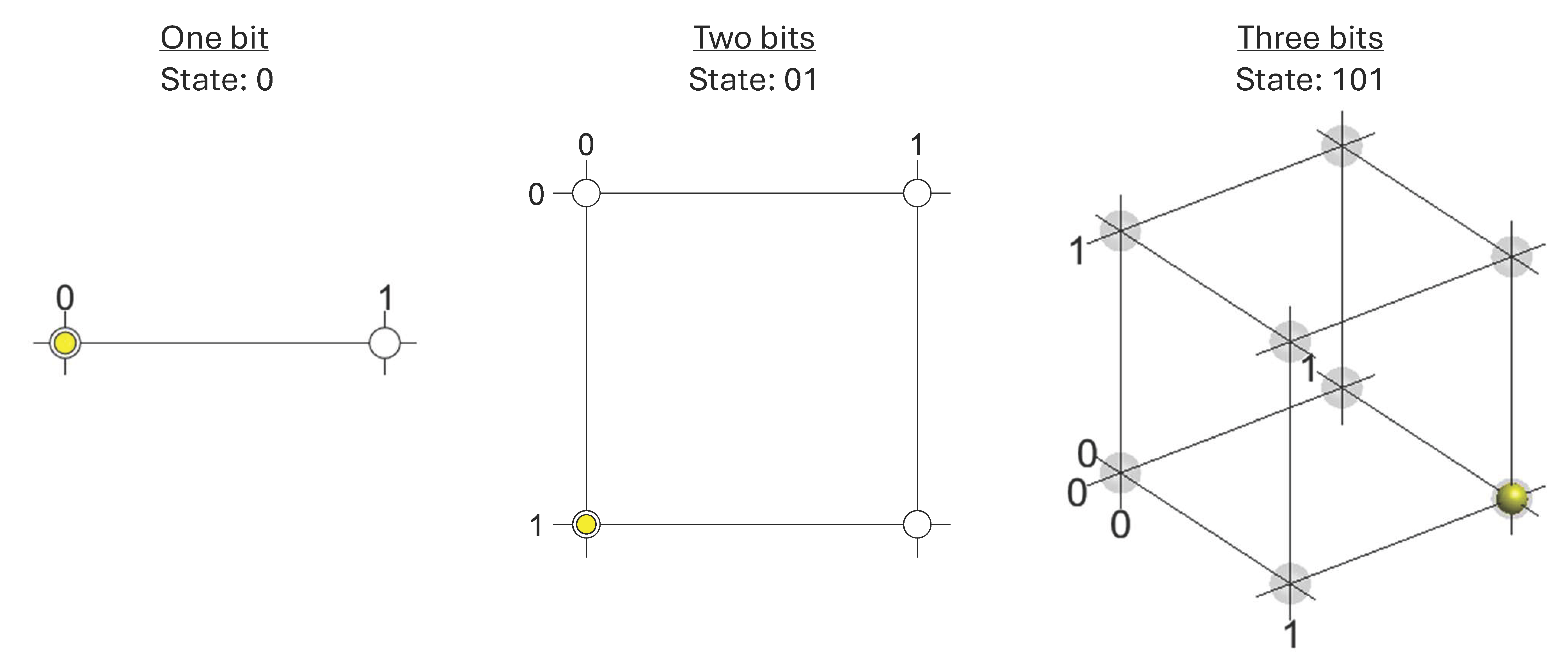
If we add a second bit, we can indicate its two possible states in a direction perpendicular to the first. This yields four possible states for the two-bit system, “00”, “01”, “10”, and “11”. At any given time, the state of both bits can be shown by filling in a single dot at the appropriate corner of the square.

How about adding a third bit? Again, we can indicate its two possible states along a direction perpendicular to the first two. Now we have a diagram that looks like a cube, with eight possible states at the corners. We could label these states “000”, “001”, “010”, “011”, “100”, “101”, “110”, and “111”. If you are familiar with binary numbers, you will recognize that we could also label the corners with numbers 0 to 7.

As we add more bits, we keep adding more dimensions the cube, resulting in an \(N\)-dimensional hypercube. This is very hard to visualize directly, but we can get the idea from following the pattern outlined above: two points along a line extend to become four points at the corners of a square, which extend to become eight points at the corners of a cube. These 8 points at the corners of a cube then extend (into a conceptual 4th spatial dimension) to become 16 points at the corners of a 4-d hypercube. Those 16 points then extend to become 32 points at the corners of a 5-d hypercube, and so on.

Therefore, the possible states of \(N\) bits can be viewed as the \(2^N\) corners of an \(N\) dimensional hypercube. At any given time, we can fill in a dot at one of those corners to represent the state. That is, the state of the system can be specified by some number between 0 and \(2^N-1\).

Now, quantum information

Now let’s compare to the quantum case. If you have read Catland up to this point, the pictures shown in Fig. QC.1 may look familiar. They resemble the way we have visualized the quantum wave function of particles described by wave packets in two possible positions. For example, a single particle may be described by a wave packet centered at position A or position B, or a superposition of the two. If we add a second particle which may be at position C or D, then we have seen that we must visualize the wave function using a 2D plot, as in Fig. 2.1 and Fig. 2.2. This yields a plot with blobs positioned at the corners of a rectangle with vertices \((A,C)\), \((A,D)\), \((B,C)\), and \((B,D)\). One possible state of the two particles would a single blob at one of the corners, as shown at the left of Fig. 2.1. But now the key difference between the quantum and classical state: the quantum wave function may be a superposition of blobs at any number of the corners. Moreover, those different blobs may have different amplitudes and different phase differences between them. This is why the quantum state contains more information than the corresponding classical state. In the classical case, the state is specified by indicating which single corner represents the state; in the quantum case, an amplitude and phase must be specified for all \(2^N\) corners.

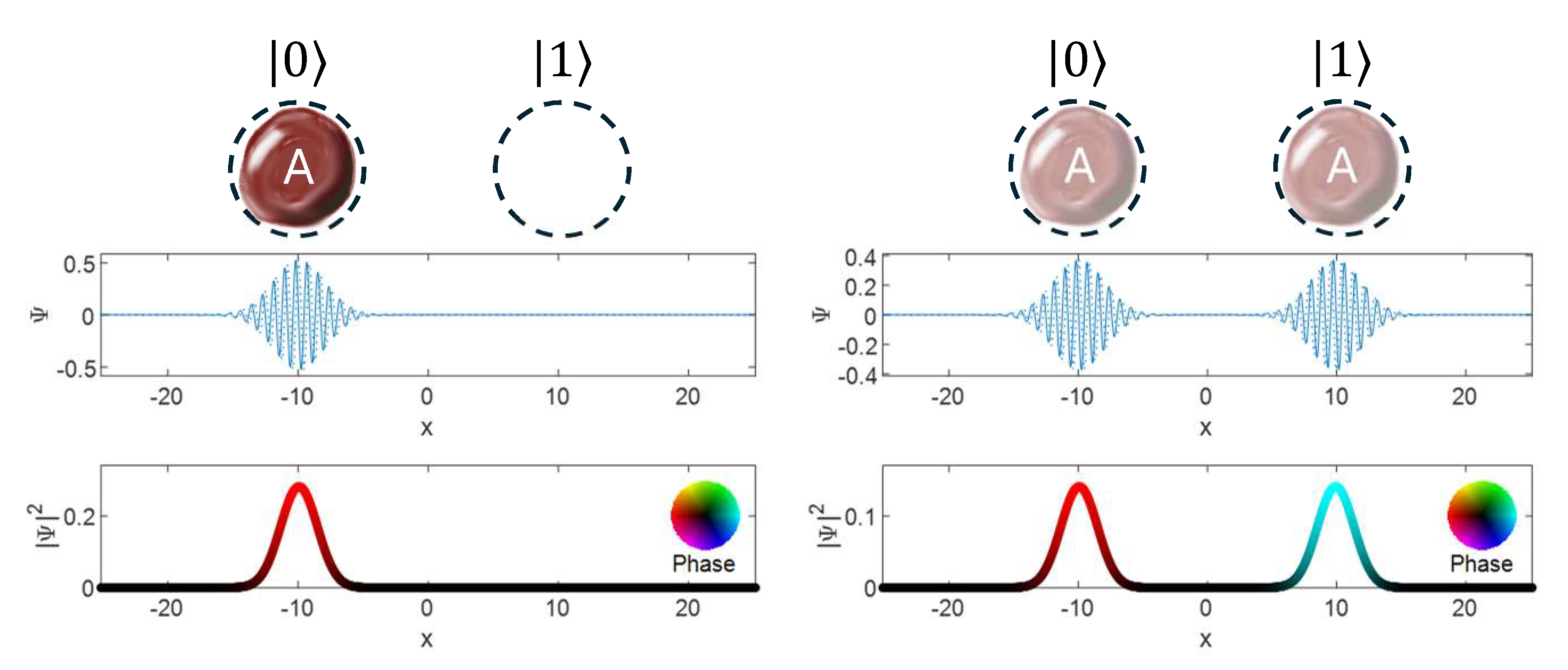
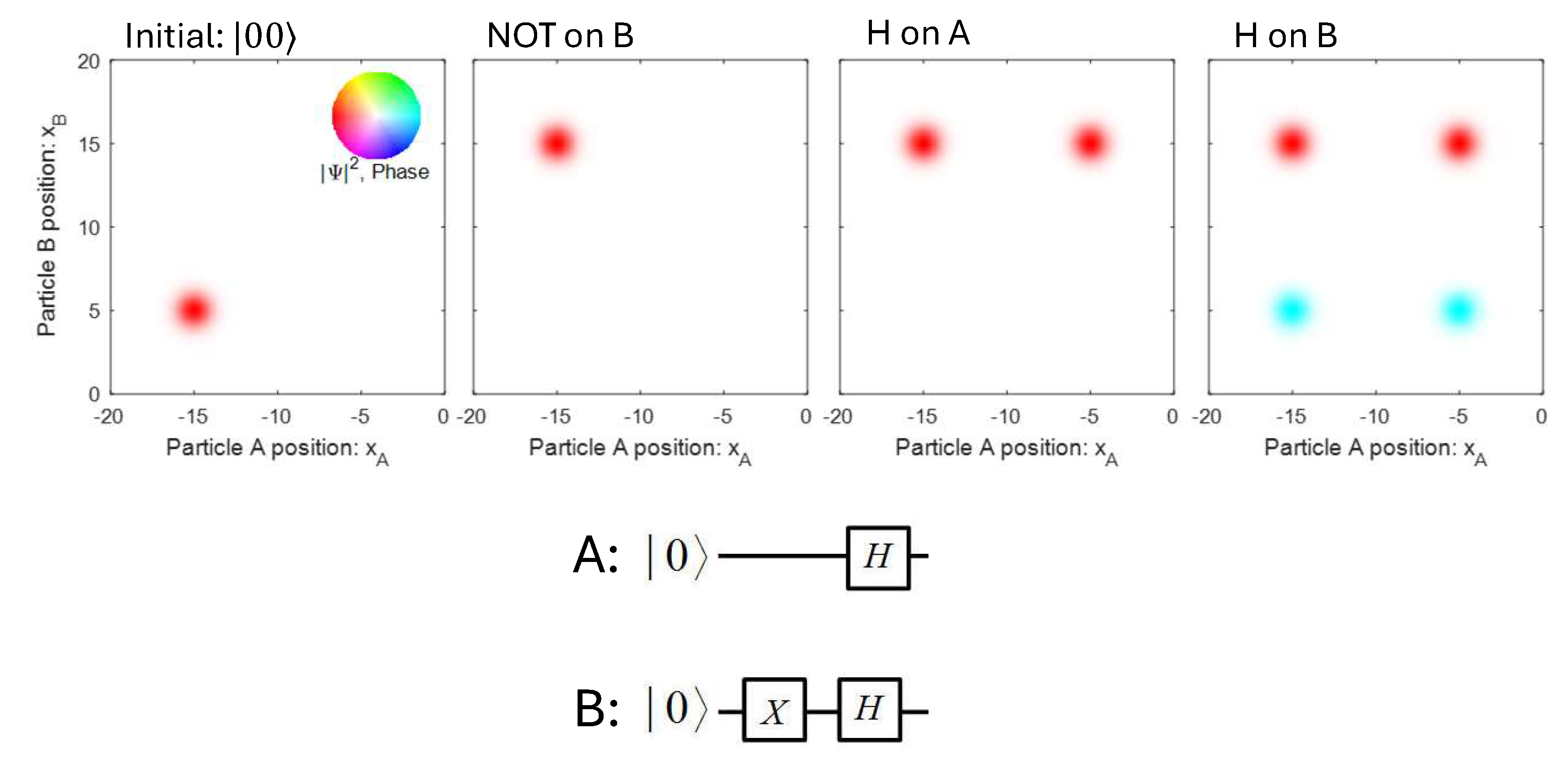
In the quantum example here, each particle is called a “qubit” (quantum bit). In general, a qubit is a quantum system with two well-defined states that can be designated \(|0\rangle\) and \(|1\rangle\). In this example, a wave packet in one position could be \(|0\rangle\) and a wave packet in another position could be \(|1\rangle\), as illustrated in Fig. QC.2. A cartoon representation is shown by the red ball labeled “A,” which can occupy one or both of the dashed circles. At the left, we see the qubit state \(|0\rangle\), and at the right, we see a superposition of \(|0\rangle\) and \(|1\rangle\). Because we can not only specify the amplitude of the wave function for both packets, but also the phase difference between them, we have color coded the bottom plot of the amplitude squared to indicate the phase of the wave, according to the color wheel in the inset. Though the overall phase is arbitrary, we can see that the two packets at the right of Fig. QC.2 have opposite phase, as their colors are opposite on the color wheel.

Figure QC.2

States of a single qubit. Particle A can be described by a wave packet in one of two positions, or in a superposition of both. The left position is called state \(|0\rangle\) and the right position is \(|1\rangle\). The red ball shows a cartoon of particle A occupying one or both positions. The plots show the actual wave function, with the real and imaginary parts plotted at the top, and the amplitude squared at the bottom, colored to show the phase of the wave function relative to a reference wave.

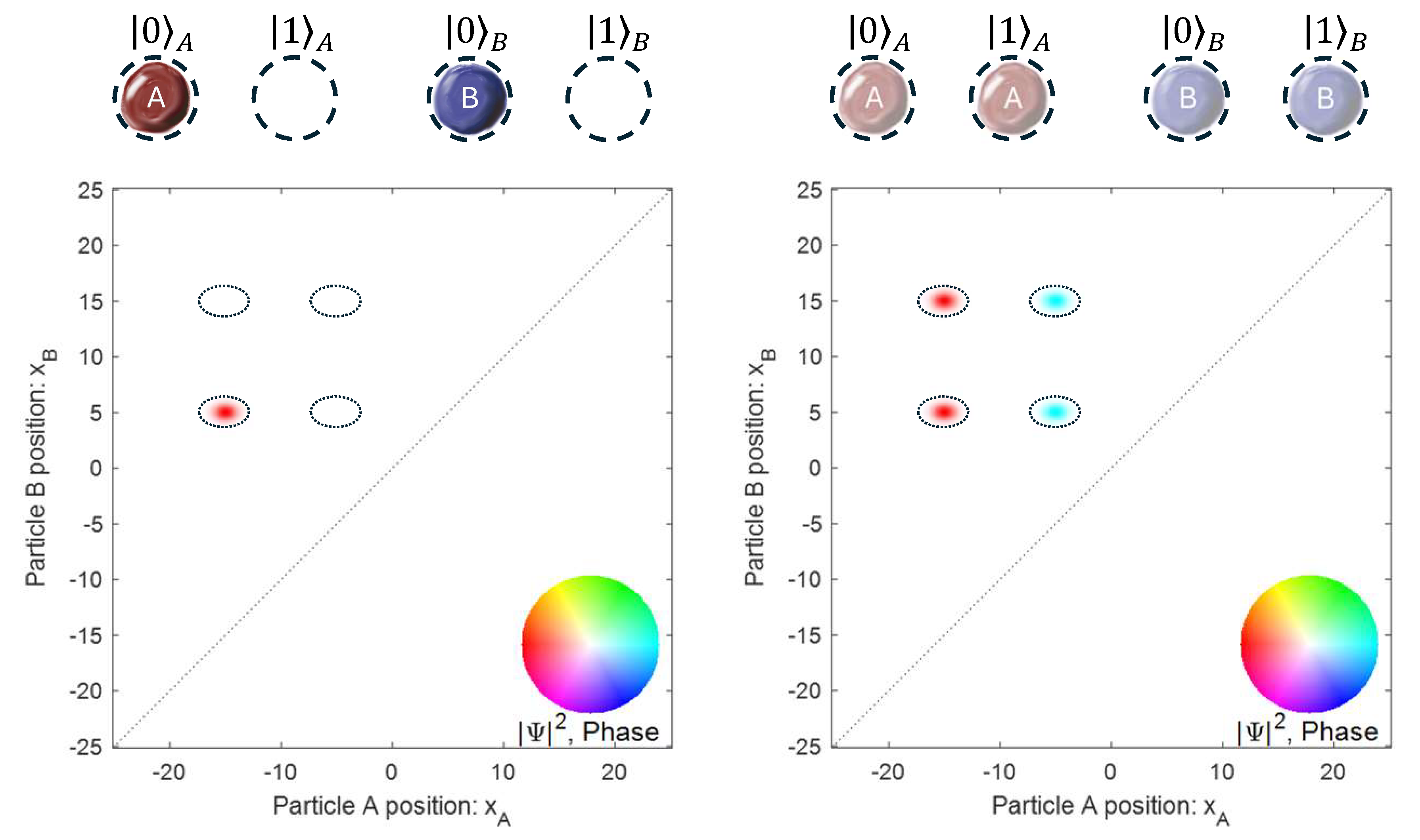
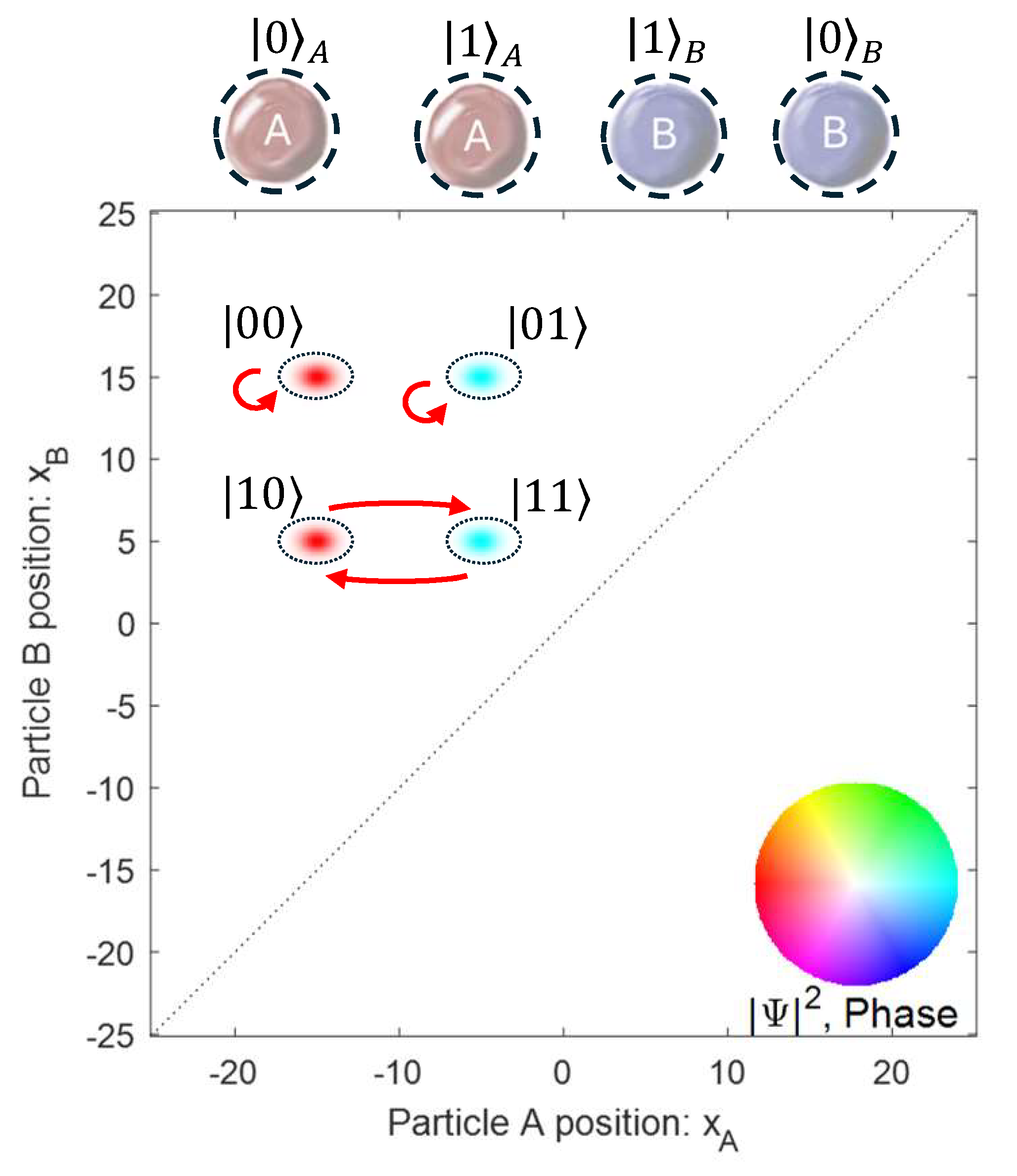
With two qubits (two particles), then the wave function is represented by a superposition of the four states in the 2D plane, \(|00\rangle\), \(|01\rangle\), \(|10\rangle\), and \(|11\rangle\). Two example states are shown in Fig. QC.3. At the left, the state \(|00\rangle\) is shown, as drawn in the cartoon as particle A and B both in their “0” positions. In the 2D plot of the two-particle wave function, a single blob shows Particle A at \(x=-15\), and Particle B at \(x=5\). The four possible locations of blobs are indicated by dotted ellipses. At the right, we see a two-qubit state where both particles are in a superposition of their two locations. Particle A is at both \(x=-15\) and \(x=-5\) and Particle B is at \(x=5\) and \(x=15\). This results in four blobs in the 2D plot of the wave function. As an example, we have set the two components of particle A to have opposite phase, and the two components of particle B to have the same phase. This is shown by the color coding of the blobs in the plot of amplitude squared.

Figure QC.3

States of two qubits. Particle A and Particle B can both be described by a wave packet in one of two positions, or in a superposition of both. The left position is called state \(|0\rangle\) and the right position is \(|1\rangle\). The red and blue balls show a cartoon of particle A and B occupying one or both of their positions. The plots show the actual wave function, with amplitude squared colored to show the phase of the wave function relative to a reference wave.

We have also seen an example that could be interpreted as three qubits, such as the three-particle case in Fig. 6.2. Here, the state must be visualized in 3D, with each axis corresponding to the 1D position of one of the particles. Now there are eight distinct qubit states, each represented by a blob at one corner of a 3D cube. But again, the state in general can be a superposition of these blobs with different amplitudes and phase differences. In this way, the \(N\)-dimensional wave function for \(N\) particles moving in one dimension looks directly like the \(N\)-dimensional hypercube we used to visualize \(N\)-bit systems above.

Processing information

Once we have a set of bits or qubits storing some information, we can process that information to perform a computation. We can think of the initial state as an input, and the final state as an output.

Processing classical information

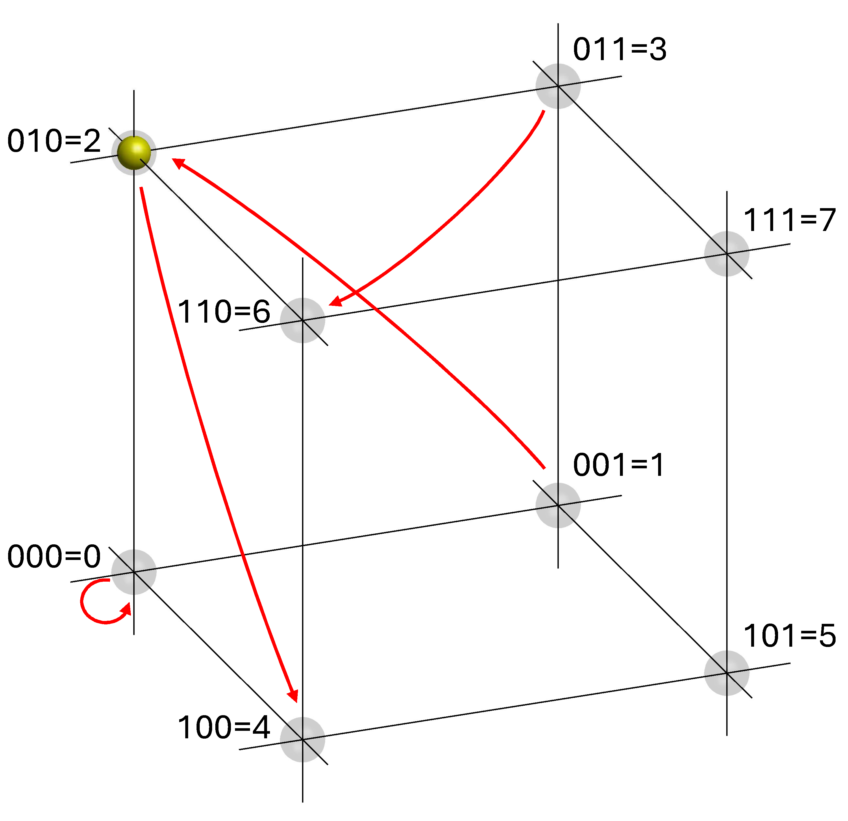
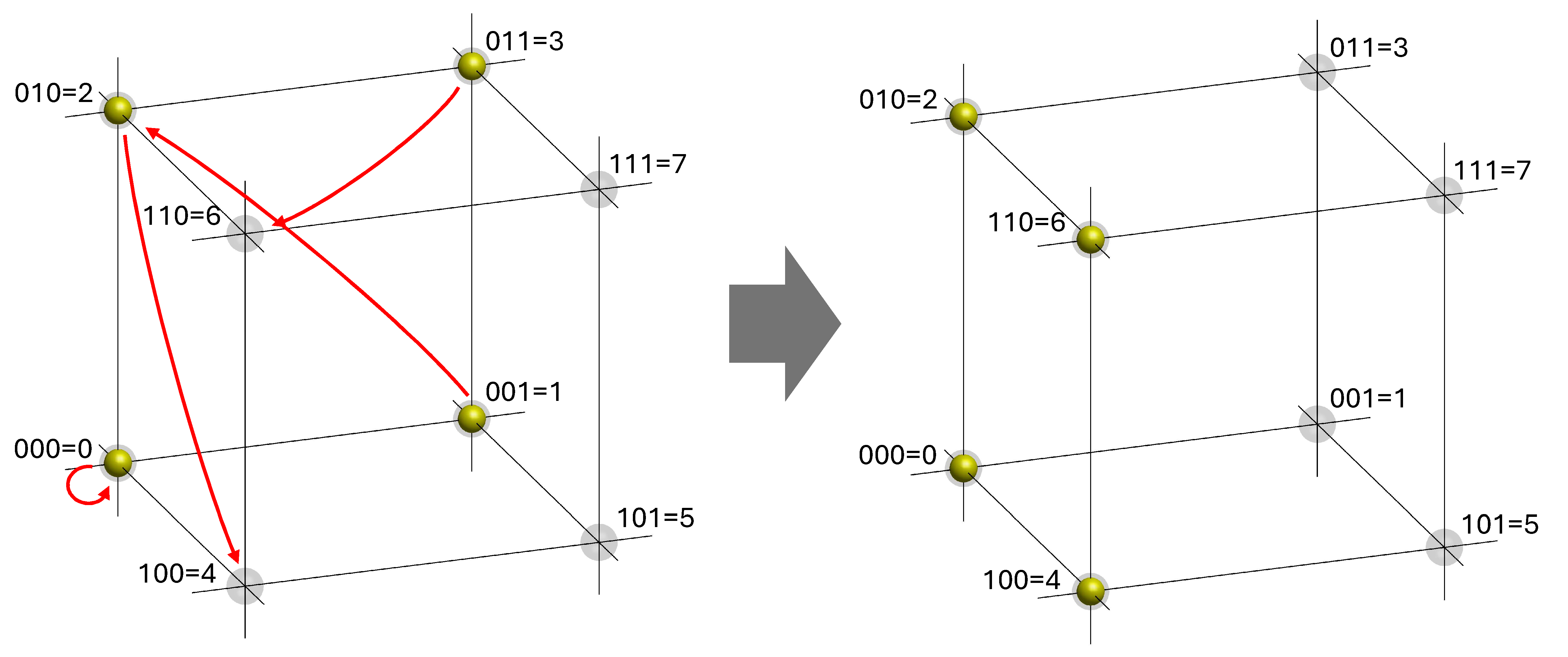
Let’s start again with the classical case. Say we have 3 bits, so the initial state is represented by a dot at one corner of a cube. We could interpret the eight possible initial states as an input 0-7. Then we want to process that information to, say, multiply the input by 2. We’ll restrict the inputs to be 0-3, so we have enough bits to represent the output of 0, 2, 4, or 6.

The action of this operation is shown in Fig. QC.4. Given any initial state of the system, bits will be flipped so as to result in the desired final state, as indicated by the red arrows.

Figure QC.4

Visualization of a classical computation that takes an integer input 0-3, and outputs the input multiplied by two.

So how to build such a device in practice? We could try to come up with some contraption or electronic circuit that would perform the desired operations on each input as shown. But this would be difficult to come up with, and not generalizable to larger systems. Instead, the trick of digital electronics is to break things down into very simple basic operations, then build them up to do progressively more complex computations. These operations are called “gate operations.” For example, a NOT gate operates on a single bit and has the function of flipping the state from 0 to 1 or vice versa, as illustrated at the left of Fig. QC.5.

Figure QC.5

Visualization of classical gates. Red arrows indicate how the input is transformed into the output.

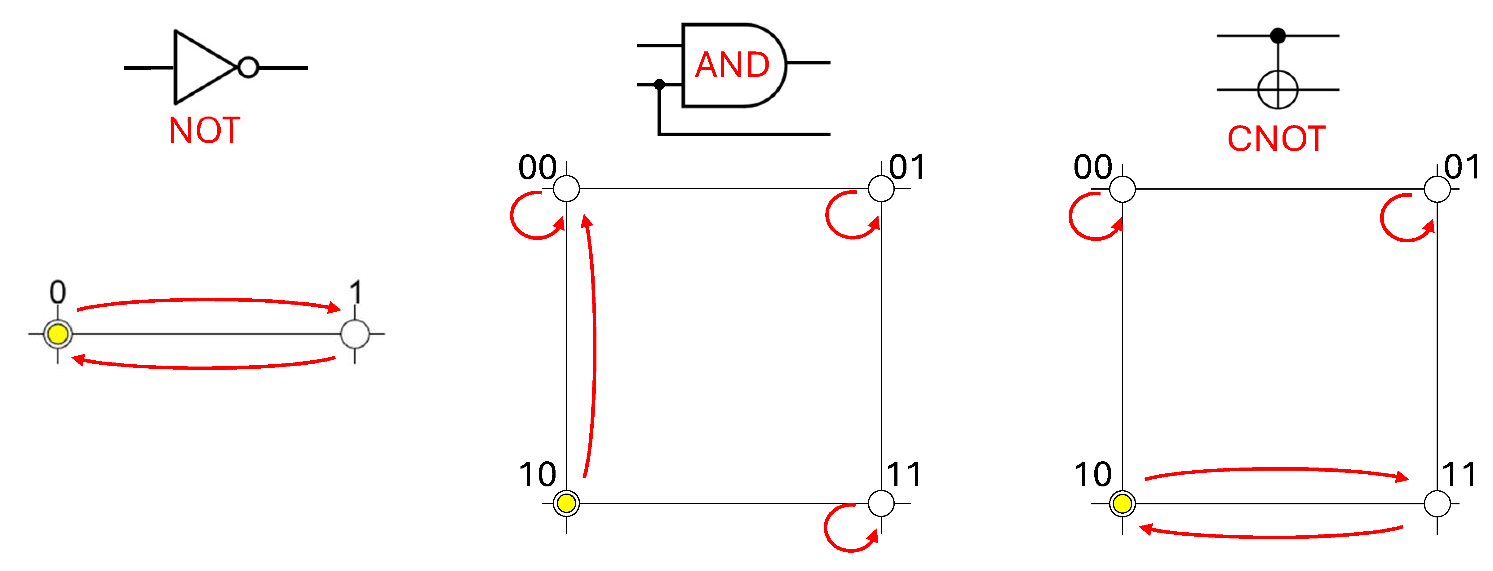
Other gates operate on two-bit inputs. In digital electronics, it is often the case that the number of input and output bits are not the same, which complicates the visualization of the state on a hypercube. For the sake of simplicity, we will assume that the number of input and output bits are the same. For example, the standard AND gate takes two bits as an input, and yields a single bit as an output. If both input bits are 1s, then the output is a 1. Otherwise, the output is a zero. However, we can illustrate this with two output bits by putting the actual output in the first output bit, and leaving the second input bit as the second output bit. This is illustrated in the middle of Fig. QC.5.

As a final example of a two-bit classical gate, we illustrate the controlled-NOT, or CNOT gate (right of Fig. QC.5). The first bit is the “control” bit: if it is 0, then nothing is done to the second bit, but if it is a 1, then the second bit is flipped (a NOT operation is performed on it). The control bit is unaffected, and the first input is the same as the first output bit.

From just a small number of elementary gate operations, any computation can be built up by stringing them together in the appropriate way.

Now we will turn to the quantum case: how can we use quantum gate operations to perform a computation on the quantum information in a set of qubits?

Processing quantum information (the wrong way)

Before seeing how it works, let’s first examine an idea that doesn’t work. We could envision the classical computation shown in Fig. QC.4 but now as a system of three qubits. We can still envision the state of the system as a 3-D cube, but now instead of the state being just one corner at a time, the wave function can have amplitude at multiple corners simultaneously. This suggests the idea that instead of just putting one input in and doubling it, we could simultaneously put in all the inputs 0-3 and double them all at once. Indeed, we could carry out this process, illustrated in Fig. QC.6. At the left, the wave function has amplitude at inputs 0, 1, 2 and 3, which is then transformed to the state on the right with amplitude at 0, 2, 4, and 6. The catch, however, is what happens when we try to amplify the information in this quantum system up to a scale that would be perceptible to a human.

Figure QC.6

Visualization of a system of three qubits, initially in a state with equal amplitude at states 0-3, transformed into a state where each input state is doubled so as to have amplitude at states 0, 2, 4, and 6.

A general issue that must be confronted in quantum computing is that the qubits must typically be microscopic so as to avoid decoherence during the computation, but then the quantum state must ultimately be amplified in some way so that we can find out what it is. This is precisely the issue discussed in the Amplification and decoherence section.

To take a look at the final state at the right of Fig. QC.6, note that such a state may be non-entangled and thought of as two particles (A and B) in a superposition of their 0 and 1 packets and a third particle (C) in its zero packet. Focusing on, say, qubit A, how can we perform a micromeasurement to determine the state? That is, how can we have a new particle come in, interact with this qubit, and wind up in a state that depends in some way on the qubit’s state?

One way to perform a micromeasurement, discussed at length throughout Catland, is to collide a particle described by a single wave packet off of our qubit. (The idea of this position micromeasurement is first introduced in the Double slit section.) The result will be an entangled state with two components. One where the incoming particle has collided with the qubit at the 0 position, and one where the incoming particle has collided with the qubit at the 1 position. If we want to visualize this new wave function, we must add a new dimension to the plot to take into account the probe particle. If the position information has been unambiguously transferred, then the two blobs of the original superposition will now be misaligned along the probe particle’s position axis.

To get to the macroscopic scale, many more such microscopic interactions must occur. These may be more particles interacting with the original qubit, or a cascade of interactions following from the probe particle(s) (see, for example, the “marble run” device in the Amplification and decoherence section). Furthermore, as the system size approaches the macroscale, accidental interactions with particles in the environment (i.e. decoherence) become more and more likely. Each such interaction that transfers the position information will result in the blobs being separated along more and more dimensions.

Finally, we can safely say that any further system that interacts with these blobs will only do so in a way that depends on each blob separately, and does not depend on the existence or location of the other blob. The only way for this assumption to fail is if two blobs become re-aligned along every dimension (possibly on the order of \(10^{20}\)) and interfere with each other. Ultimately, you are a system that must interact with the blobs, if you wish to perceive them. The above argument says that your wave function will now have two components, one corresponding to you perceiving the qubit in one location, the other corresponding to you perceiving the qubit in the other location. That is, there is a “version” of you that measures the qubit to be in the 0 state, and another version that measures the qubit to be in the 1 state.

Returning now to the three qubit system, we can apply the same reasoning to understand what we will perceive for all three qubits. Referring to the diagram in Fig. QC.6, we’ll refer to the first number in the binary string as qubit A, the second as qubit B, and the third as qubit C. The state of qubit A separates front from back in the diagram. The state of qubit B separates top from bottom, and qubit C separates left from right.

Since the qubits are not entangled in this example, we can surely consider them separately. So first, probe particles are used to amplify the state of qubit A, resulting in the two versions of you perceiving the state of qubit A to be 0 and 1. There are still four yellow blobs, as in Fig. QC.6, but the pair of blobs at the front and the pair of blobs at the back are now separated along a huge number of dimensions. Each pair remains aligned in the vertical direction, but there is extremely little chance of them ever coming back into alignment in the front-to-back direction.

Next, probe particles interact with qubit B, which is also in a superposition of 0 and 1 as represented by the vertical pair of blobs in both parts of the wave function. Now the blobs in each pair get separated along a further huge number of dimensions. When you ultimately interact with the probe particles, there are now four distinct parts of the wave function: one each where you perceive the two qubits in the states 00, 01, 10 and 11.

Finally, probe particles interact with qubit C. This one is not in a superposition of packet locations, as shown in Fig. QC.6. It is only in the 0 location. Therefore, when the probe particles collide with this qubit, there remains just a single blob along the left-right axis. So all parts of the wave function record a state of 0 for qubit C.

After all three qubits have been measured, the wave function now contains 4 separate parts. They are separate because they are misaligned along so many dimensions that it is extremely improbable that they will ever overlap and thereby interfere with each other. In such a case, it is safe to consider each part separately, as if the others do not exist. In the four parts, the three qubits are seen to have the values of 000, 010, 100, and 110, corresponding to integers 0, 2, 4, and 6.

The upshot is that after measuring all three qubits, there are effectively four versions of you, one seeing the number 0, one seeing 2, one seeing 4, and one seeing 6. If the four blobs originally had equal amplitude, then you will perceive these outcomes as occurring with equal probability (see Born’s Rule). What we have accomplished then is a fancy random number generator that yields one of four even numbers at random.

While generating random numbers using quantum effects may have some practical use for cryptography, it is not what we want if we are trying to use a quantum system to perform computations.

This example highlights a central requirement for quantum algorithms: not only must the quantum system perform a computation, but the result must be accessible even after amplification to the macroscopic scale. That is, all versions of you must be able to successfully obtain the result of the computation. We will see below how this is possible, though only in certain cases.

Quantum gate operations

Just as with classical computing, it will be useful to define elementary quantum gate operations that allow us to perform basic operations on one or two qubits at a time. Then these operations can be strung together to perform any more complicated operation. We’ll now take a look at how these operations can be implemented on our wave packet qubits.

Most simply, we will want to be able to move packets from one location to another. For a single qubit, this will allow us to make the quantum version of the NOT gate described above in the classical case. Physically, we could implement such gates by applying local electric fields if the particles are charged, or colliding the qubit with other (much heavier) particles that repel the qubit particles. These other particles must be much heavier to avoid recoil and thus unintended entanglement. This was discussed in the Double slit section, where in Fig 3.3 a much heavier particle acts as a passive mirror. Likewise, whatever system is used to apply local electric fields would need to do so passively, without becoming entangled with the qubit. This is one of the challenges of building quantum computing devices: fast and precise control over the qubits’ state is required, but must be implemented in a way that does not introduce any unwanted entanglement (i.e. decoherence).

The effect of the NOT gate is demonstrated in Fig QC.7. For the sake of an interesting example, the initial state of the qubit is an out-of-phase superposition of the 0 and 1 packets with different amplitudes. The effect of the gate is to swap the two packets. When the two packets overlap, they interfere with each other, though this has no lasting effect in this case: the two packets just continue on their way after crossing.

Figure QC.7

Video example of the single qubit NOT gate, operating on a state in a superposition of two wave packets.

In the same way that we can move the packets around to implement the NOT gate, we will further assume that we have the capability to move individual packets around at will, again say, by applying local electric fields. As long as a packet is not spatially overlapping any other packet, we should be able to apply a force locally to move it. Conversely, if two packets are overlapping spatially then we can only apply the same force to both. So for example, in the state shown at the right of Fig. QC.3 with all four blobs present, applying a force at \(x=-15\) could be used to move the two red blobs right or left, but not to move them separately. The capability to move packets around at will is needed to keep the packets in the designated “0” and “1” locations after operations, as we will see below.

In addition to the quantum analog of the classical NOT gate, the extra degrees of freedom in the quantum case require additional single-qubit gates. Specifically, we need gates to control the degree of superposition between 0 and 1, and the phase between 0 and 1.

We can implement a phase gate by altering the speed (and frequency) of one of the packets for a fixed time. In particular, we can apply a local attractive potential that will increase a packet’s speed and frequency as the packet passes by. If we design the potential cleverly, the particle can pass by with a phase shift, with no reflection (the so-called sech-squared potential). The phase gate is demonstrated in Fig. QC.8. Here, the initial state is a qubit in a superposition of two out-of-phase packets. The applied potential is shown as the red dashed line. Once the left packet has passed the dip in the potential, the phase has been changed by 180 degrees (\(\pi\) radians). Note that in the final state, the packets are no longer in their designated “0” and “1” positions. At this point, we can turn off the phase-shifting potential and use our ability to move the packets around to put them back to their original positions.

Figure QC.8

Video example of the single qubit phase gate, operating on a state in a superposition of two wave packets. The packets are initially out-of-phase, and the gate changes the state to be in phase.

Last but not least of the single-qubit gates will be one to take a single packet and make a superposition, or vice versa. In the quantum computing lingo, this is called a Hadamard gate. This gate will again use something we have seen before – a beamsplitter. An external potential that acts to split a single packet into two was first shown in Catland in the context of Klein-Gordon waves back in the Classical waves section (Fig. 1.5). Later, the same effect was shown in Fig. 3.2 in the Double slit section where the beamsplitter is implemented as a second much heavier particle with a weak repulsive interaction.

Here we will implement the Hadamard gate by again assuming we have a way of switching on an external potential. The potential in this case will be a very narrow potential barrier near \(x=0\). By changing the height and/or width of this potential, we can set the transmission and reflection to be 50/50 (or any other ratio if desired.) The effect of the gate is shown in Fig. QC.9, for an initial state \(|0\rangle\) (packet on the left). As desired, the single packet splits into an equal superposition of packets on the left and right.

Figure QC.9

Video example of the Hadamard gate, operating on a state initially in the “0” packet.

The trick to setting up the Hadamard gate is that the potential barrier is offset from the midpoint of the two packets by a quarter of a wavelength. This makes the two final packets above have the same phase. On the other hand, if we started in the state \(|1\rangle\) (packet on the right), the two packets end up out of phase after the Hadamard operation. And all of these operations work the same way in reverse: an in-phase superposition overlappping at the origin results in an outgoing packet to the left, and an out-of-phase superposition results in an outgoing packet to the right. All four of these situations are shown in Fig. QC.10.

Figure QC.10

Video example of the Hadamard gate operating on four initial states.

The phase-dependent behavior of the Hadamard gate is a crucial feature for quantum computing. In the examples here, we see that the Hadamard gate serves to translate position information into phase information, and back again. The action of the Hadamard gate can be viewed as a result of wave interference. For example, when two packets meet at the central barrier, their transmitted and reflected packets can interfere either constructively or destructively to result in a single packet either moving to the right or left. This will be an important tool in taking the result of a quantum computation and translating it into a state that we can perceive classically.

Now we can turn to two-qubit operations. The only two-qubit operation we will need is the quantum analog of the controlled-NOT (CNOT) gate shown in the classical case above. The action of the CNOT gate is to either flip or not flip the state of one bit (the target), depending on the state of the other bit (the control). In Fig. QC.5, the state of a two bit system was depicted as one corner of a square, and the CNOT gate leaves the top two corners alone while swapping the state in the bottom two corners. Our quantum implementation will be the same, but with a two-particle wave function with wave packet components that may be at the corners of a square, as shown in Fig. QC.11. As indicated by the red arrows, any packets at the top two corners will be left alone, and those at the bottom two corners will be swapped. In this example, after the CNOT operation the bottom left blob would be cyan and the bottom right blob would be red.

Figure QC.11

Example of a two qubit wave function with the operation of the CNOT gate illustrated by the red arrows.

The key to implementing a quantum CNOT gate is that it generally involves interaction between two qubits that can alter the entanglement of the state. For example, if want to swap the two lower blobs in Fig. QC.11 and leave the upper two in place, we cannot do that by applying local forces to the packets. If we try to move the lower left blob to the right (along the \(x_A\) axis), the upper left blob also moves to the right. That is because these two blobs derive from the same Particle A packet – if we apply an external force to one, we are by definition applying the same external force to the other.

The way around this is to move the packets via an interaction between the two particles. Such an interaction can generate entanglement, as has been discussed at length throughout Catland. The generation of entanglement by the collision of two particles was first shown in Fig. 2.6. Here we will follow the same setup: the two particles interact only at a very short distance, where they strongly repel each other. They essentially bounce off each other like billiard balls.

To perform the CNOT operation, we will make use of the collision to misalign the blobs, allowing us to further manipulate them using locally applied forces. The procedure will be as follows:

1. Use local forces to increase the separation of the control qubit packets, bringing the “1” packet of the control qubit nearer to the target qubit.

2. Use local forces to launch the two qubits towards each other.

3. Allow both packets of the target qubit to collide with the nearer “1” packet of the control qubit.

4. Before the far “0” packet of the control qubit collides with the target, use local forces to realign all of the now-separated blobs to their designated positions according to the CNOT scheme.

These steps are illustrated in Fig. QC.12. In this example, the initial state is an equal superposition of both qubits in both locations, all with the same phase. This yields the four red blobs shown in the initial state at the left. Step 1 is to move the \(|0\rangle_B\) packet of particle B farther to the right, as shown in the cartoon at the top. This is because particle B is the control qubit, and we don’t want the part of the state correlated with \(|0\rangle_B\) to be swapped. In the plot of the wave function on the left, this results in the blobs forming a tall rectangle, since the position of particle B is shown on the vertical axis. The four blobs are labeled by the corresponding states of B and A, with B listed first as is traditional for the control qubit.

Figure QC.12

Illustration of the scheme for performing a quantum CNOT gate.

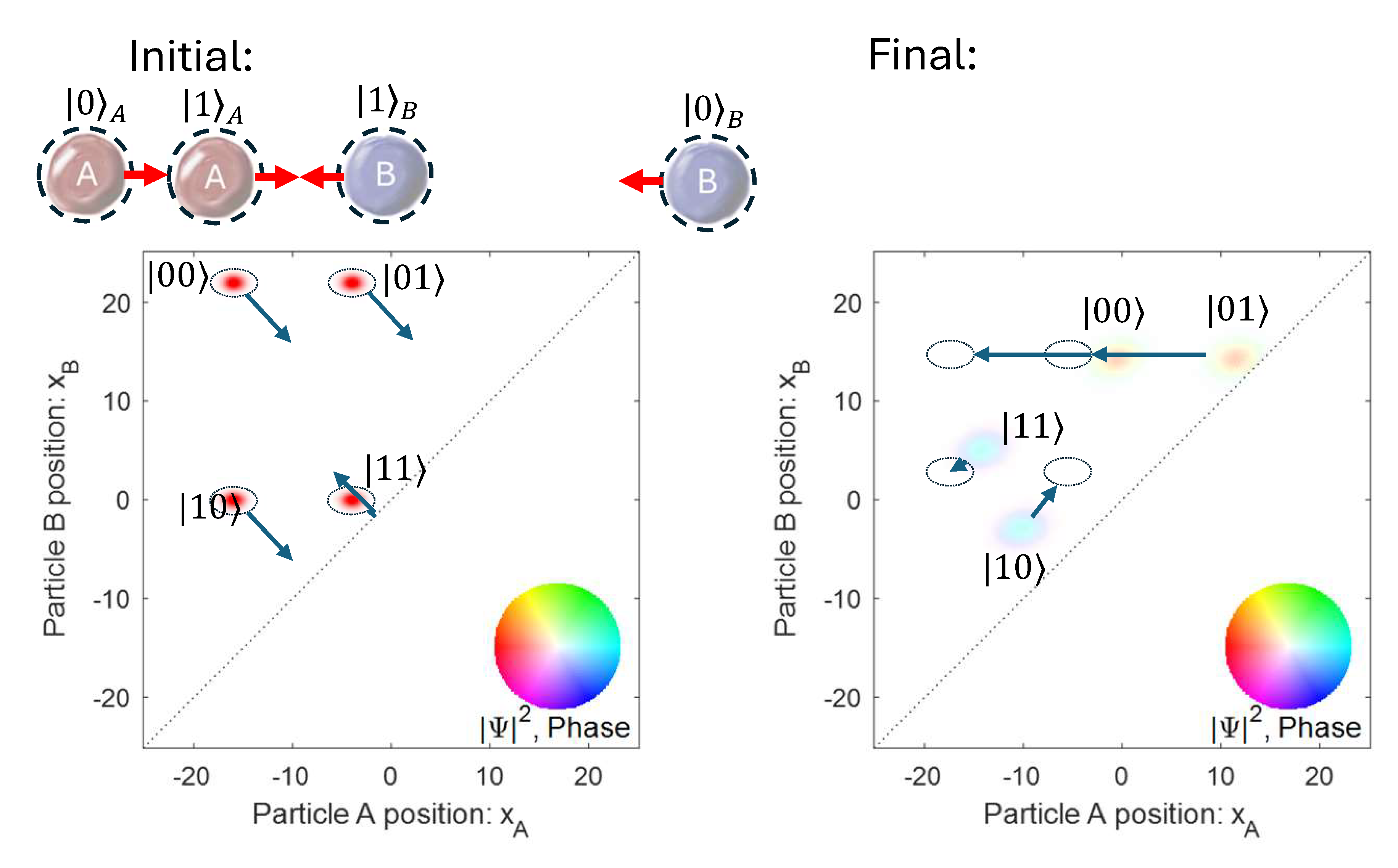
We then launch particle A and B towards each other (step 2). In Fig. QC.12, this is shown by the red arrows in the cartoon, and also by the blue arrows in the plot of the wave function. Two particles collide when they reach the dotted diagonal line. This is where the \(x\) coordinate of one particle equals the \(x\) coordinate of the other. So particles moving towards each other are shown by a blob moving toward the central diagonal, and particles moving away from each other are shown by a blob moving away from the central diagonal. As is indicated by the blue arrows, the first part of the wave function to collide will be the \(|11\rangle\) blob, at which point it starts moving back away from the central diagonal. Then the \(|10\rangle\) blob will collide next. The state on the right shows the wave function at this point, when \(|11\rangle\) and \(|10\rangle\) have collided but \(|01\rangle\) and \(|00\rangle\) have not. The evolution from the initial state on the left to the final state on the right is shown in video form in Fig. QC.13. At this point, step 3 is completed.

Figure QC.13

Video example of the CNOT gate operating on an initial state with equal superposition of all two-qubit basis states. The CNOT operation is then completed by shifting the phase of the lower two blobs by \(\pi\) and moving the packets back into the square arrangement.

Next, we will use locally applied potentials to put the packets into their designated positions as zeros and ones of two qubits (step 4). This is now possible because the collision has rendered the blobs to all be misaligned. We will also need to apply a \(\pi\) phase shift to the \(|11\rangle\) and \(|10\rangle\) packets to correct for the phase shift they acquired during the collision. The repositioning of the packets is shown by the blue arrows in the plot at the right of Fig. QC.12. The blobs are labeled the same as in the initial plot on the left. Note that the \(|11\rangle\) and \(|10\rangle\) blobs will now be swapped.

The CNOT gate has the capability to take an initial non-entangled state, and transform it into a final entangled state. For example, the initial state with the control qubit in a superposition of \(|0\rangle_B\) and \(|1\rangle_B\), and the target qubit in the state \(|0\rangle_A\) could be plotted as two vertically aligned blobs. The action of the CNOT gate would be to reflect the lower of the two blobs, but not the upper thus swapping the position of the lower blob. The resulting entangled state would be two misaligned blobs, one in the \(|00\rangle\) state, and one in the \(|11\rangle\) state.

Deutsch’s algorithm

With the quantum gate operations now in hand, we will now look at a first example of a quantum algorithm, Deutsch’s algorithm, which demonstrates an advantage over the classical case. Deutsch’s algorithm is a classic example of a quantum algorithm. It is not intended to be practically useful, but instead to serve as a minimal example.

The premise of Deutsch’s algorithm can be described as follows. Someone hands you a black box capable of performing an unknown computation that takes one bit as its input (0 or 1) and yields one bit as its output (0 or 1). We would like to answer the question: do both inputs yield the same output (both 0 or both 1), or do the two inputs yield different outputs (one 0 and one 1)?

If the box is performing a classical computation, then it is straightforward to see how to answer the question. Just try both inputs and see what the results are. First, plug a 0 into the input. The answer will be 0 or 1. Next, plug a 1 into the input. Either the output matches the first output or it doesn’t. Voilà.

The important thing in this simple example is that in the classical case, we have to use the black box twice, putting in the inputs one at a time. But perhaps if we can somehow put in both inputs at once, we can get this information in one go? Let’s see.

As before, first we’ll look at an idea that doesn’t work. One way that our quantum black box might work is by implementing one of four possible single-qubit operations on the input qubit to yield the output. Note that there are four possible actions of the box: for the inputs \((0,1)\), the outputs could be \((0,0)\), \((1,1)\), \((1,0)\) or \((0,1)\). We are trying to distinguish the first two from the last two.

For example, the black box could send the two packets of the input qubit towards each other as if performing a NOT operation. But then a strong, reflecting barrier could be placed in front of neither, one, or both of the packets. No barrier in front of a packet (and that packet’s transmission) could be considered a 0 output for that input, and the presence of a barrier (and that packet’s reflection) could be considered a 1 output.

After the input packets have either been reflected or transmitted, the information about the corresponding outputs is contained in the state. Certainly, if we only put in one input packet (the input is either 0 or 1, but not a superposition) we can find out the corresponding output by looking at the final position of the packet. This is just the classical case though, requiring two runs to answer the question. What if we put in both inputs at once as a superposition?

If we start with a particle in the “0” packet, we can transform it into a superposition using the Hadamard gate, as described above. The black box will now send both packets towards the origin, both either reflecting off of a barrier or not, depending on the action of the box. Fig. QC.14 shows the four possible wave functions evolving from the input to the output. The red dashed lines show the presence or absence of reflecting barriers that set which outputs are generated.

Figure QC.14

Video example showing the four possible cases of Deutsch’s algorithm, where the output is determined by the presence or absence of a reflecting barrier.

The final states shown in Fig. QC.14 are indeed different, depending on the four different sets of outputs of the box. Each packet could now be labeled as “inner” or “outer” depending on whether it was transmitted and is now close to the origin, or whether it was reflected and is now farther from the origin. But we have to be careful – in reality we don’t get to look at a plot of the wave function. We must next amplify the result to the macroscopic scale so we can perceive it. As usual, we will use a position micromeasurement in which we collide a probe particle with the qubit particle. In each of the four cases, this will result in a two-particle entangled state which could be plotted in 2D as two misaligned blobs. Each blob will represent the probe particle correlated with the position of one of the two qubit packet positions. We then can amplify the micromeasurement, for example, using the marble run device. As discussed above, this results in the two blobs becoming misaligned in so many dimensions that we can henceforth safely consider the two blobs separately. The end result, as before, is that there will be two versions of you, one perceiving the qubit to be at the position of one packet, and another version seeing the qubit at the position of the other packet. So in the case of output \((0,0)\), there would be one version of you seeing a packet around \(x=-3\) and another version seeing a packet around \(x=+3\). Each version of you has only learned about one output. Neither version of you has enough information to tell whether the action of the box is to output \((0,0)\) or either \((0,1)\) or \((1,0)\). This is just the same as in the classical case. The quantum case has gained us nothing.

But wait, besides the positions of the packets, there is another feature of the final states in Fig. QC.14 that distinguishes between the two cases of interest. It is the phase difference between the two packets of the qubit. The \((0,0)\) and \((1,1)\) cases have zero phase difference, whereas the \((0,1)\) and \((1,0)\) cases have opposite phase. This occurs because a packet picks up a \(\pi\) phase shift when it reflects. What we want to do then is to amplify the phase information, instead of the position information. Or if we want to use our nice apparatus we already built for measuring position information, we can just convert the phase information into position information. For this, we can use the Hadamard gate. If we take the final state in any of the four cases and apply a Hadamard gate, the result is shown in the bottom two panels of Fig. QC.10. A phase difference of zero results in a single packet going to the left, and phase difference of \(\pi\) results in a single packet going to the right. Now if we perform the position micromeasurement and amplification, there is only one packet so only one result for us to perceive. If we perceive a packet going to the left, we know that the output of the box is \((0,0)\) or \((1,1)\); if we perceive a packet going to the right, we know the output is \((0,1)\) or \((1,0)\).

We have now successfully extracted perceptible information about the black box using a single run, which would have taken two runs classically. Note that though the input was a superposition of both inputs, in the end we do not learn the value of even a single output. Instead, we learn a different, single piece of information. So it’s not that the larger amount of quantum information allowed us to perceive a result with a larger amount of information. Instead, we were able to manipulate the quantum information in such a way as to render a different piece of information classically perceptible, than would have been possible using classical information alone. The trick was to take the whole quantum state (in this case, of just a single qubit) and use interference to transfer information about the whole state into the classically perceptible position of a packet.

Deutsch’s algorithm another way

In the example above, we looked at a particular implementation of the black box, where the output is given by either reflecting a wave packet, or not. In general, implementations of Deutsch’s algorithm follow the same scheme. A Hadamard gate puts the qubit into a superposition state. Then somehow, the action of the black box flips the phase of either component of the superposition if the corresponding output is a “1”. Then a Hadamard gate reveals the phase difference between the two components.

A more common version of Deutsch’s algorithm uses a second qubit to achieve the phase flips. We’ll take a look at that next. In this case, one qubit is still the input and the other qubit is just an extra, or “ancilla.”

The first few steps of the single-qubit-plus-ancilla version of Deutsch’s algorithm are shown in Fig. QC.15. Qubit A will be the input qubit, and qubit B will be the ancilla. The first panel shows the initial state of \(|00\rangle\), which is a single blob at the lower left. That is, both qubits are in their leftwards location. As shown in the diagram at the bottom, we then apply a NOT operation to qubit B, flipping it to its “1” location. Next we apply a Hadamard gate to both qubits. Taking them one at a time, the Hadamard applied to qubit A results in two in-phase blobs separated along the \(x_A\) axis. Next, the Hadamard applied to qubit B splits both of the existing blobs in two, resulting in four blobs. Since qubit B was starting from the “1” position, the Hadamard gate splits the blobs into out-of-phase pairs.

Figure QC.15

The first three steps of Deutsch’s algorithm, with a single qubit input (A) and an ancilla qubit (B).

Starting from the final panel of Fig. QC.15, the next step is to encode the output of the black box. The idea here is to flip the packets of qubit B correlated with any input state of A that yields an output of 1. These operations are shown in the first column of Fig. QC.16. If the outputs are \((0,0)\), then we flip nothing. If the outputs are \((1,1)\), then we flip both pairs of B packets. That is, we just perform a NOT gate on qubit B.

Figure QC.16

The remainder of Deutsch’s algorithm, for all possible outputs with a single qubit input (A) and an ancilla qubit (B).

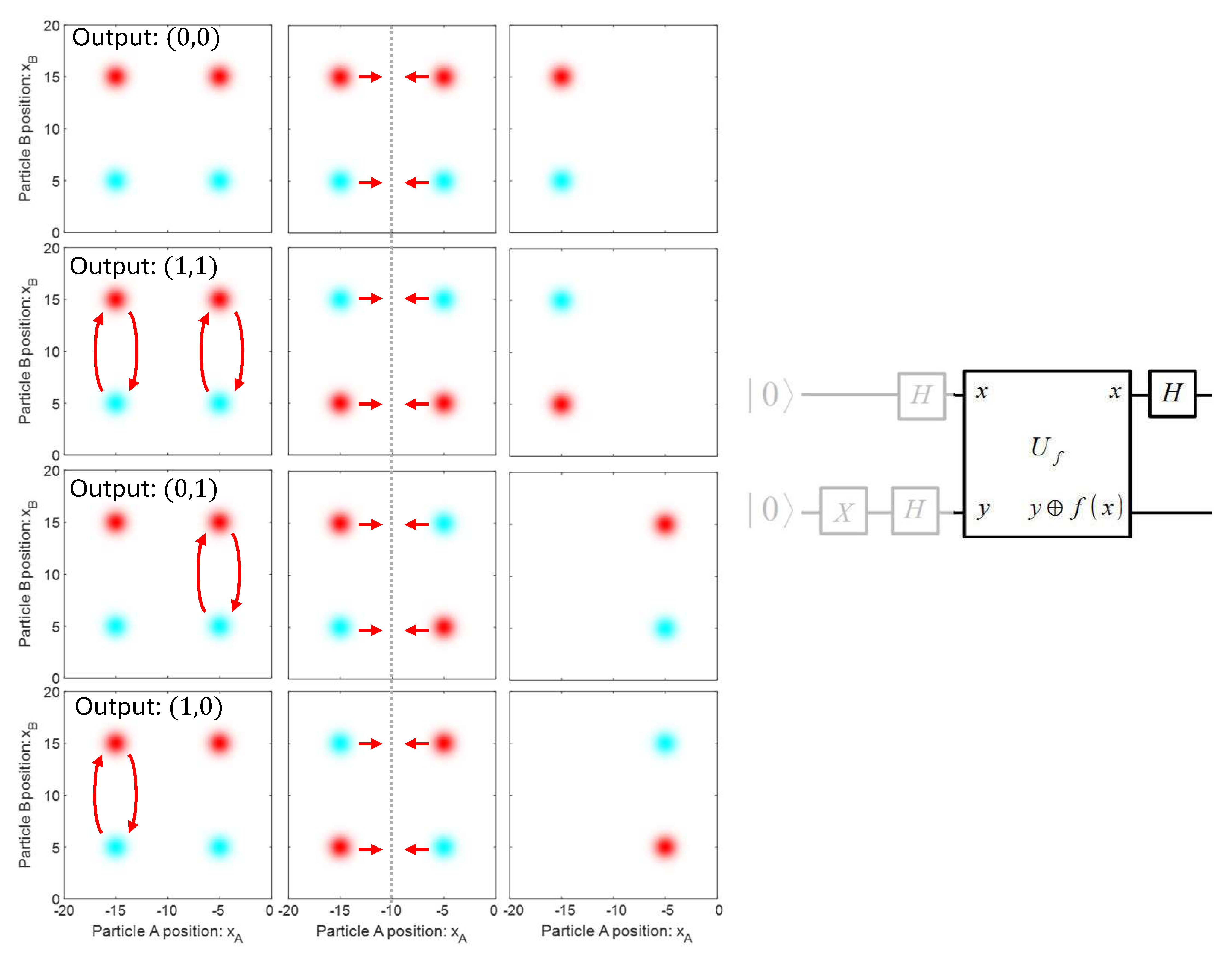
The bottom two operations shown in the first column of Fig. QC.16 are a little trickier. Here, we want to just flip the packets of B that are correlated with one of the states of A. But this is just like the CNOT gate discussed above. The resulting states are shown in the second column, all with four blobs but different patterns of their phases. We now have four different quantum states corresponding to the four different possible box outputs. But again, we cannot just read off the quantum state – we have to do some further manipulation to get our result into a form that can be amplified and perceived at the macroscopic scale.

The final step is to apply a Hadamard gate to qubit A. In our implementation, this means sending both of particle A’s packets towards the origin in the \(x_A\) direction, with a beamsplitter placed so as to distinguish between in-phase and out-of-phase packets. In-phase packets combine into a single packet that goes back to the “0” location, and out-of-phase packets combine into a single packet that goes to the “1” location. In the top two rows, we see that the combined packets are all in-phase, so they all wind up at Particle A’s “0” location. On the other hand, in the lower two rows, all the combined packets are out-of-phase, so they all wind up at Particle A’s “1” location.

At this point, we have arranged the situation so that the difference of \((0,0)\) or \((1,1)\) vs. \((0,1)\) or \((1,0)\) is directly encoded into the position of particle A. We can now perform a position micromeasurement on particle A, and amplify. Since there is just one location for particle A, we perceive just that position for particle A. The result of this measurement reveals whether the outputs of the box are the same, or different. Note that we don’t need to measure particle B. We can if we want, but we don’t gain any information – it is the same in all four cases up to an arbitrary phase shift.

This implementation of Deutsch’s algorithm highlights an interesting aspect of quantum information processing. The action of the black box seems to be applied only to qubit B, but in the end the perceptible change is to qubit A. Indeed, in the top two rows of Fig. QC.16, we haven’t done anything to qubit A. We either perform a NOT operation or do nothing to qubit B, but qubit A just remains as an in-phase pair, which combines back together via the Hadamard gate to return to its original “0” state. It wouldn’t matter if qubit B is even on the same planet as qubit A in this case. It’s the bottom two cases where something more subtle is going on. Here, we flip packets of qubit B only correlated with certain positions of qubit A. As we saw with the CNOT gate, now the two qubits must come together and interact. It is here that our classical intuition breaks down, and we really need to think of the system as being described by a two-particle wave function.

A nice aspect of this implementation of Deutsch’s algorithm is that it can be extended to inputs of more than one qubit. This generalization is often known as the Deutsch-Jozsa algorithm, which we will turn to in the next section.

The Deutsch-Jozsa algorithm

In Deutsch’s algorithm above, we had a black box with one-qubit input and outputs, and we saw that we could find something out about it in one shot that would have taken two shots classically. Now we will generalize this to a black box with \(N\) input bits and one output bit, and see that we can find out something in one shot that would take \(2^{N-1}+1\) shots. That is much more impressive!

So now our black box will have \(N\) input bits or qubits. We can think of the collective input as an \(N\)-digit binary string, or a number between 0 and \(2^N-1\) (or a superposition of these in the quantum case.) For each individual input, the box will yield an output of either 0 or 1. The possible outputs of the box will be limited to cases where either all outputs are the same (all 1s or all 0s), or half of the inputs yield a 0 and half yield a 1. These two cases are referred to as “constant” and “balanced.” As before, the goal will be to determine whether the output of the box is constant or balanced.

First, we can look at the classical case. In this case, we have no option other than putting in inputs one at a time. So how many times do we need to plug inputs into the box to determine whether it is constant or balanced? Let’s say there are \(N=100\) input bits. We could plug in an input at random, corresponding to a number between 0 and \(2^{100}-1\) (a very large number). The output will be 0 or 1. Let’s say that the output was 0. At this point, of course we have no idea whether this will be a constant output of 0, or a balanced output where half will be 0 and half 1. Then we put in another input at random. Say the output is 0 again. This could still be either a constant output of zero, or maybe we just happened to hit two of the 0s of a balanced output. Say we keep plugging in inputs, and keep getting zeros. We still can’t be sure whether the output will be all zeros, or if we are just (luckily or unluckily) hitting repeated zeros of a balanced output. We can only be sure once we have tried out more than half the possible inputs. If, at this point, all the outputs have been zero, then we have ruled out the possibility of a balanced function since if that were the case we would have had a 1 by now for sure. Half the possible inputs comes to \(2^{99}\), which is also a really enormous number. This is the number you need to try to be assured that you will have a definitive answer. Of course, you might find out that the function is balanced sooner, but it will take at least two tries before you can know anything.

Turning to the quantum case, we will see that as before, we need just a single run to determine whether the output is constant or balanced. The procedure will be exactly the same as the single-bit input with ancilla, but now with more input bits. Now we will have \(N\) input qubits, plus one ancilla qubit. The initial state will be all qubits in the zero state. Imagine a long line of \(N+1\) particles, each of which is a wave packet in the left of two possible locations. The wave function of these particles can be visualized as a single blob in a \((N+1)\)-dimensional space. We first apply a NOT gate to the ancilla qubit. This means we move the ancilla particle’s packet to the rightward location. The blob correspondingly is shifted along the axis corresponding to that particle’s position.

Now we take that single blob, and apply a Hadamard gate to all \((N+1)\) qubits. Taking them one at a time, the evolution of the wave function is just the same as how we described the construction of an \((N+1)\)-dimensional hypercube above. First, the blob splits into two along the axis of the first qubit. Then those two split along the axis of the second qubit to form a square. Then those 4 blobs split along the a third axis to form 8 blobs at the corner of a cube, then 16 blobs in 4-d, then 32 blobs in 5-d, and so on. If we save the ancilla qubit for last, then all of the Hadamard gates until then are coming from the “0” location, so result in packets with the same phase. Then when we apply the Hadamard to the ancilla (which remember was shifted to the “1” location), the \(2^N\) blobs split into out-of-phase pairs, resulting in two \(N\)-d hypercubes, with opposite phase, separated along the ancilla qubit’s axis.

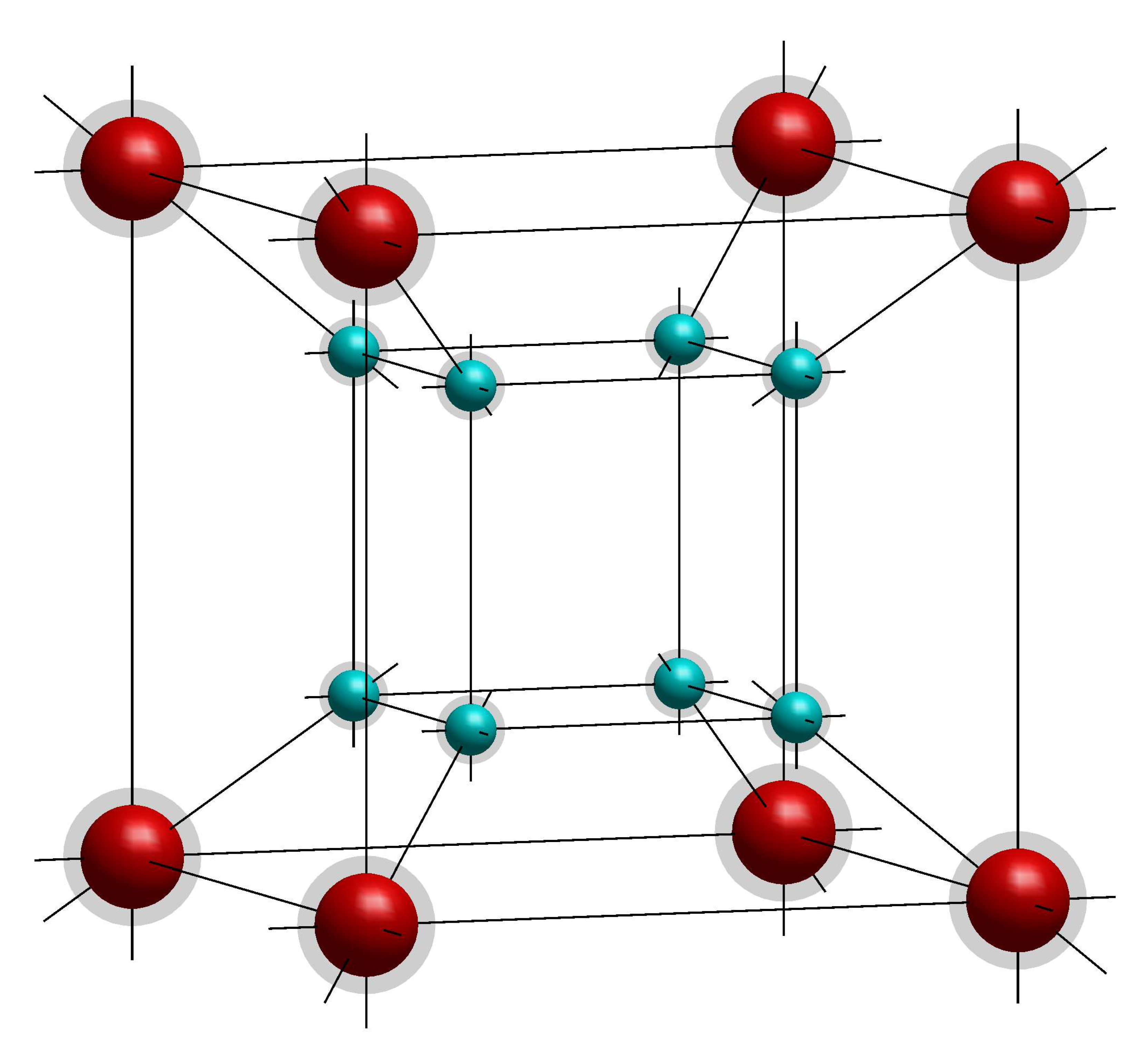
Fig. QC.17 shows a visualization of this state for \(N=3\). The three input qubits plus one ancilla qubit require a 4D plot to visualize the wave function. This is somewhat difficult to visualize. The key is to view the inner cube not as an actually smaller cube, but as an equal-sized cube that appears smaller due to the effect of perspective as it is farther away in the 4th dimension. In this case, I have foregone actually simulating a real wave function, and instead am drawing spheres to replicate what the wave function would look like. The spheres are color coded as above to indicate the phase of different blobs. The red blobs represent the 8 possible 3-bit inputs correlated with the “0” packet of the ancilla, and the blue blobs with the “1” packet of the ancilla.

Figure QC.17

Illustration of wave function for the Deutsch-Jozsa algorithm with three input qubits and one ancilla, showing the state after Hadamard gates have been applied to all qubits.

To simplify a bit, we will go forward with an example in the case of \(N=2\). The wave function is illustrated at the left of Fig. QC.18. The two input qubits plus one ancilla qubit require a 3D plot to visualize the wave function. In these plots, the left-right and top-bottom axes represent the position of the two input qubits wave packets, and the front-back axis represents the ancilla qubit’s packet locations. The four input states are labeled. As expected, the input qubits’ state consists of an all-in-phase square of blobs representing all four inputs. The two out-of-phase packets of the ancilla result in two copies of this square that are out-of-phase with each other.

Figure QC.18

Illustration of wave functions for the Deutsch-Jozsa algorithm with two input qubits and one ancilla. Left figure shows the state after Hadamard gates have been applied to all qubits. Middle and right figures show the state after conditional NOT operations representing two possible balanced outputs.

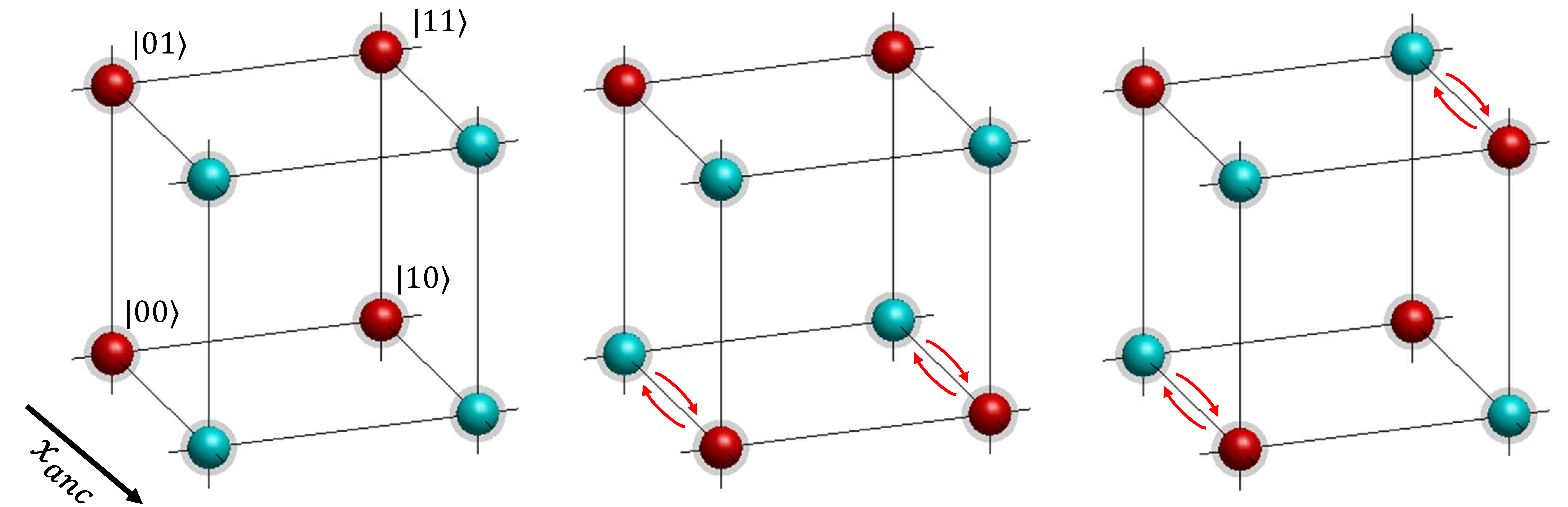
Next, we want to perform a NOT operation on the parts of the ancilla qubit correlated with any inputs that yield a “1” output. The result will be to flip the phase of any blobs corresponding to “1” outputs. In the example shown in Fig. QC.18, there are 8 possible sets of outputs. Two are constant: all 0s or all 1s. These are encoded either by leaving the original, leftmost plot alone, or by performing a NOT gate on the ancilla qubit, swapping all the blues and reds. Two of the six possible balanced output cases are shown in the middle and right of Fig. QC.18. The middle plot shows the case where \(|00\rangle\) and \(|10\rangle\) inputs yield an output of 1. The right plot shows the case where the \(|00\rangle\) and \(|11\rangle\) inputs yield an output of 1. The other four cases are similar.

After this step, all the outputs of the black box are encoded in the state, and now it is time to manipulate the state so we can obtain a macroscopically perceptible result. This is accomplished by applying a Hadamard gate to all input qubits. Referring to the example in Fig. QC.18, we can visualize the Hadamard gate on the first input qubit as moving the left and right faces of the cube towards each other, and placing a beamsplitter near the midpoint where the blobs will interfere. Recall what happens: when two in-phase blobs come in, a single blob of the same phase goes back to the “0” side; when two out-of-phase blobs come in, a single blob matching the phase of the transmitted blob goes to the “1” side. So after this first Hadamard gate, there will be just one blob along each of the four left-right edges. The position of those blobs (left vs. right) will depend on whether the blobs that met were in-phase or out-of-phase. Next, the Hadamard gate is applied to the second qubit. That operation can be visualized as combining the blobs at the top of the cube with their partners at the bottom, and placing a beamsplitter in the appropriate location where they interfere.

So what does the final state look like, after these Hadamard operations? First of all, note that the front and back faces, corresponding to the two states of the ancilla qubit, are always the same but with opposite phase. So the Hadamard operations along the input qubit axes have the same effect for both front and back planes. The situation is particularly simple for the constant output cases. Here, all the blobs that meet during the Hadamard operations are in-phase, so the blobs always go to the “0” side. After both operations, we have just two blobs, both correlated with the \(|00\rangle\) state of the inputs (and both states of the ancilla). This result is the same for any number of inputs, in fact. The second round of Hadamard gates essentially just undoes the first round of Hadamard gates, returning us to the original state of the input qubits \(|00\rangle\).

The situation is a little more complicated in the case of balanced outputs. Looking at the examples at the middle and right of Fig. QC.18, we can trace what happens. In the middle, the left-right blobs are in phase, so the blobs all go to the “0” side on the left. Those blobs will be out-of-phase in the vertical direction, so will go to the “1” side at the top. This results in two blobs, both correlated with the \(|01\rangle\) state of the inputs (and both states of the ancilla). In the case on the right, we can see that both Hadamard operations will involve out-of-phase pairs. So first we obtain all blobs at the right-most “1” state. Those blobs will be out-of-phase in the vertical direction, so will then go to the “1” side at the top. This results in two blobs, both correlated with the \(|11\rangle\) state of the inputs (and both states of the ancilla).

If we go to higher \(N\), the final state in the balanced cases can be more complicated to determine. In general, there can be many blobs at many corners of the hypercube. But there is always one thing we can say for certain: it will never have any amplitude for the \(|00...0\rangle\) state of the input qubits. This happens because of the symmetry of the balanced outputs. No matter which balanced case you choose, the interference will always ensure that the amplitudes cancel out for the \(|00...0\rangle\) state.

So now let’s think about what happens when you perform position micromeasurements, and amplify. We will collide a probe particle with each of the input qubit particles. (We don’t care about the ancilla qubit, so we leave it alone.) The case of constant outputs is particularly simple. In this case, the input qubits only have a single blob at \(|00...0\rangle\). Therefore, each probe particle collides with each input qubit at the “0” location, with no resulting entanglement. Further amplification reinforces this result, ultimately allowing you to perceive the result of “0”.

What we perceive in the case of balanced outputs is a little more complicated, because now there can be many blobs at different corners of the hypercube (though not at the \(|00...0\rangle\) corner). Now a probe particle will become entangled with any input qubit in a superposition of its two locations. This will result in the blobs correlated with the two states of that qubit axis to become separated along a new dimension. As that micromeasurement is amplified, the misalignment spreads to many, many more dimensions. Ultimately, the \(N\) micromeasurements and amplifications result in complete misalignment of all blobs at any of the \(2^N\) corners of the input qubits’ hypercube. Since none of these blobs have any realistic chance of interfering again, we can safely consider their future evolution as occurring as if the other blobs don’t exist. Applying the same logic as above, that means that you will perceive different outcomes of the measurements corresponding to each input with nonzero amplitude.

So to summarize: if the black box output is constant, you only perceive the qubits to be in the state “0”; if the output is balanced, there are many versions of you perceiving different qubit states, but none of them are the “0” state. We can now see that whichever version we find ourselves in, we can answer the original question of whether the black box output is constant or balanced. If you perceive “0”, it is constant; if you perceive something other than “0” it is balanced.

Quantum vs. classical

Some questions that may arise include: why is there one set of rules for classical bits and a different set of rules for quantum bits? Why can’t we perform quantum gate operations on classical bits? Why can’t we make quantum bits large enough that we don’t need to amplify the final state, and can just observe them directly?

The answers to these questions come down to the phenomenon of decoherence. Decoherence occurs when there are accidental interactions between the bits or qubits and some other systems in the environment. Just as in the intentional process of micromeausurements and amplification, this leads to entanglement between the qubits and particles in the environment. The only difference is that it happens in an uncontrolled way, and we may not be able to access these environmental particles that have become entangled with our system.

Let’s imagine what would happen if we tried to make our qubits macroscopic. We could imagine that the wave packets represent the position of a marble. Our qubit could be a short segment of track along which the marble can roll. At either end of the segment is a divot where the marble can sit. The marble in one divot represents “0”, and in the other divot, “1”. Various mechanisms could launch the marble from one divot to the other. For example, mechanisms at both ends of the segment could be activated to launch the marble to the other divot. This would implement a NOT gate – whichever side the marble is on, it will get launched to the other side. These mechanisms could be triggered by the position of another marble on a different track, implementing a CNOT gate.

Somewhat more strange is to consider what happens if we try to do something phase-dependent, like a Hadamard gate. Following our previous Hadamard implementation, we should place a partially transmissive barrier near the midpoint of the marble track. When the marble rolls across this barrier, its wave function should be split in two, with one packet continuing on and the other reflecting back. This is certainly counter to our classical intuition. There are several issues here. One issue is that the barrier walls must be narrow compared to the wavelength of the wave function. Otherwise, the wave function either reflects or is transmitted like one would expect for a classical particle. For a typical marble, this wavelength is extremely small. But for the sake of this discussion, let’s set aside this problem, and assume we can somehow create such a barrier.

Then if the marble starts in the “0” divot and rolls across the barrier, we end up with the marble sitting in a superposition of the “0” and “1” divots. This is hard to imagine. What would it look like? Would it look like a partially transparent marble in two locations, like in the cartoons in some of the figures above? I have certainly never seen anything like this before in the real world.

There is a good reason why we have never seen this before. What would have to happen for us to observe this situation? Well, a lot of photons would have to bounce off of the marble and enter our eyes. Let’s take the photons one by one. A first photon is heading toward the “0” divot position. If the marble is there, the photon will bounce off and go towards your eye. If the marble is not there, the photon will pass through and go away from your eye. If the marble has just passed through a Hadamard gate and is in a superposition of the two divot positions, the result of the photon interaction is an entangled state. In one component, the marble is in position “0” and the photon has reflected, in the other component, the marble is in position “1” and the photon has passed through the “0” position unimpeded.

We could plot the situation in 2D, initially with two blobs aligned along the marble’s position axis. The marble starts in a superposition of two locations, with the photon incoming as a single packet. The collision has essentially no effect on the motion of the marble, as the momentum transferred by a collision of a photon is far too small to deflect the marble significantly. But the different path of the photon in the two cases results in the blobs becoming very well-separated along the photon’s position axis. This effect is shown in the video in Fig. 8.7.

Next, another photon may reflect off a marble, or not, either at position “0” or “1”. This will separate the two blobs of the wave function along another dimension. As more and more photons reflect, the two blobs of the wave function become misaligned along a very large number of dimensions.

At this point, the reasoning above applies: any additional system that interacts with the system of marble + photons can only do so in a way that doesn’t depend on the existence of the other blob. To do so would require the blobs to overlap in this high-dimensional space and interfere. In other words, the evolution of one blob can never “know” about the existence of the other blob. Following this reasoning to its logical conclusion, if the new system is the wave function of your eye, your optic nerve, your brain, there must be two parts to this wave function after the interaction. One corresponding to you perceiving the marble at position “0”, one at position “1”.

This duality of perception is the same as when we performed a micromeasurement and amplified the result. Just in this case, the system being measured was already macroscopic. If we assume that this system is in an environment full of photons, the process can’t not play out. As soon as the first photon reflects off of the marble in a superposition of locations, the blobs are misaligned. And of course, this doesn’t just apply to photons. Air molecules or vibrations of atoms in the marble track would also do the trick. We see that this process, decoherence, is extraordinarily hard to avoid for a macroscopic system.

So what is the implication for our ability to do quantum computation with marbles? The same effect of decoherence that prohibits us from perceiving a marble in two locations also will cause any phase-dependent operation to fail. Consider again the initial state of a marble in a superposition of the “0” and “1” divot positions. As we saw in Deutsch’s algorithm, a key step is to take information encoded in phase differences and translate it into well-defined positions that we can perceive. This involved overlapping two packets on a beamsplitter. The resulting interference then combined the two packets into one, with the outgoing direction set by the phase difference.

But if a single photon has reflected (or not) off of the marble in one of its locations, the two blobs of the wave function are no longer aligned along the marble’s position axis. When we send them towards each other, the two blobs will not overlap and not interfere, even when the two components of the marble are at the same location. Instead, each blob of the wave function will hit the barrier separately and be split into two blobs, resulting in four non-overlapping blobs. This effect is simulated in Fig. 5.8 in the section on complementary observables.

What has happened is that the photon has essentially performed a micromeasurement of the marble’s position. After this, no further interaction with the marble alone can depend on the phase difference between the two packets. For this to happen, an interaction with both the photon and the marble would be required. If we lose track of the photon, this will be improbable. If many, many photons, air molecules, etc. do the same, we would need a particular interaction with the marble and all of these other particles for anything to depend on the phase difference. Essentially impossible.

Long story short: in the presence of decoherence, we have lost any information about the phase difference between different packets of the marble. Moreover, we are only able to perceive a single marble location. With these restrictions we are back to the picture of classical computing.

So decoherence is the big problem in building a quantum computer. And we see from the above discussion a particularly nasty catch: in general as we make the qubit bigger, decoherence gets worse. If we were just concerned about normal noise, like someone jostles the marble track and the marble accidentally switches from “0” to “1”, we could just make the marble bigger or heavier, or the divots deeper. But in terms of decoherence, a bigger marble will just be hit by more photons or air molecules. Making it heavier doesn’t help. The marble doesn’t have to recoil at all when a photon reflects off of it for the two to become completely entangled.

For this reason, many qubit implementations are microscopic, such as a single electron. It is also a good idea to find a way to store the information in the qubit in some way that is less prone to decoherence. In fact, the example here of two distinct locations of a wave packet is a really bad idea in practice. It is extremely prone to decoherence, as illustrated by the fact that a single photon bouncing off or not could ruin the whole game. In the next section, we will discuss a little about how these challenges may addressed in real quantum hardware. But first it is worth expanding on why the example here is so prone to decoherence.

The qubit states described here rely on two distinct positions. We have seen that whether intentionally performing a micromeasurement, or accidentally undergoing decoherence, information about the locations can be retained, while information about the phase differences between locations is lost. This represents the well-known idea of complementary observables: if information is obtained about some quantity, there are other quantities about which you can learn nothing.

But could we design a system where instead the phase differences are the thing we amplify learn about, while position information is lost? Not easily. (We can convert phase information to position information via a Hadamard gate then amplify that, but much harder to think of a way to amplify the phase information as phase information.) There is an inherent asymmetry between these quantities, and that is that the forces of nature depend on distance, and not on phase difference (or for that matter, momentum.) The interactions between particles can therefore be expected to distinguish between the different positions within the wave function.

This asymmetry has been implicitly assumed throughout: our plots of the wave function show relationships of position, and we assume that interactions only depend on where there is amplitude in this plot. This property of interactions is explicit in the Schrödinger equation. The interactions do not depend on phases. As far as I can tell, interactions that depend only on phase do not exist. We assume that the only way phase differences have an effect on an interaction is if the phases are converted to position information via interference, requiring overlapping parts of the wave function.

Real quantum hardware

The wave-packet based quantum computing scheme described above was intended to provide a way to visualize quantum information and how it is processed. The scheme, however, is wildly impractical. So how does it relate to more practical approaches being pursued today? Here, I will compare the wave-packet scheme to two other types of schemes based on single electrons: semiconductor quantum dots, and atom-based qubits. (Other prominent strategies include superconducting qubits, and photonic qubits, but these are less related to the above discussion.)

There are a few problems with the wave-packet-based scheme. One, mentioned above, is that storing the quantum information in spatially separated packets is very prone to decoherence. So we should find a way to encode information in a system where there are fewer ways that the environment will interact so as to distinguish between the states of our qubit. Another problem is that the wave packets as described don’t tend to stay put in their designated “0” and “1” states. They are generally moving about, and inevitably spreading out. A lot of work would have to be done corralling the wave packets back to their designated positions.

Types of qubits

Taking this second issue first, it would be better if our qubits were confined in some way, and not just allowed to fly around anywhere. This is generally the case in actual quantum hardware. If our qubit is based on an electron, we should have some structure that keeps it trapped in one of two states. This is like the marble track with divots we suggested for the macroscopic case. In fact, qubits based on semiconductor quantum dots often have a structure that is essentially a microscopic version of the marble track with divots. In these devices, voltages are applied to create local potentials that trap electrons in “divots” (these are the quantum dots). Other voltages can open channels between the quantum dots, and kick electrons from one dot to another. In other qubit implementations, we can make use of electron traps that nature has provided for us: atoms. Borrowing the somewhat crude but not wholly inaccurate model of electrons orbiting the nucleus, we can imagine instead of wave packets in two locations, two waves circling the nucleus at different radii. (Or more accurately, an electron in two different atomic orbitals.) This way we still have two distinct states of the electron’s wave function, but they are bound to the nucleus and won’t go wandering off. This sort of idea is used in so-called ion-trap qubits and neutral atom (“Rydberg”) qubits.

With the electrons now bound, we still need to make sure the information in the state is not too prone to decoherence. So even though semiconductor quantum dots give us the possibility of storing information via a confined wave packet in one location vs. another, it is still not a practical idea. In such a scheme, vibrations of atoms in the semiconductor would distinguish between the electron in two locations, leading to entanglement and decoherence. In the case of atoms, it is not too bad to use different electron orbitals to encode the information. Though different orbitals differ spatially, they largely overlap. Moreover, atoms are very small and can be very well isolated from the environment, making decoherence less of an issue. Even so, it is often advantageous to store the information in the spin of the electron, as opposed to its spatial wave function. This is the approach taken in the semiconductor quantum dots, and in many cutting-edge atomic qubits. The spatial wave function of an electron depends only very slightly on the state of the spin. So the information in the spin will be largely immune to the type of decoherence from spatially-dependent interactions described above. Instead, spins tend to interact with other particles via magnetic fields. Magnetic field effects are sometimes weak, and we can try to find ways to minimize or avoid them.

Implementing quantum gates

In addition to storing quantum information, we also need to process and measure it. In terms of processing the information via gate operations, perhaps the most interesting operations are those that can generate entanglement, such as CNOT. These require interaction between qubits. In the example above, this was achieved by colliding billiard-ball like particles. Interestingly, this is not too far off from what happens in real qubits, at least conceptually.

In both atom-based and quantum dot qubits, entangling gates are based on putting the two qubits into a situation where they repel or attract each other, with the interaction depending on the combination of states in the two qubits (“00” vs “01” vs “10” vs “11”). Unlike the wave-packet case, this repulsion doesn’t cause the particle to physically move very much, because now we are trapping them in place. Instead, it costs more energy for the system to be in some combinations of qubit states than others, enabling the state to evolve differently in the four possible states.

In quantum dot qubits, in which information is encoded in the spins of the electrons, the electrons of the two qubits are pushed together. Because the electrons are both negatively charged, they repel each other. What we need then, is for this repulsion to depend on the spin state of the electrons. This is accomplished via a rather subtle quantum effect that also gives rise to the Pauli Exclusion Principle – that two electrons with the same spin cannot have the exact same wave function. The effect in this case, called the exchange interaction, is like a weaker version of the exclusion principle. Two electrons with the same spin will tend to be farther away from each other than two electrons with opposite spin. Therefore, two electrons with the same spin will repel each other more strongly than with opposite spin. Just like the “11” state bouncing differently from the “01” state in the wave packet example, this difference in repulsion allows for the entangling action of the CNOT gate.

In trapped ion qubits, the repulsion between qubits is not from the electron itself, but from the whole positively charged ion. Again, these trapped charged particles repel each other. In this case, instead of bringing two qubits close together, we just wiggle one of them. Then the repulsive force with other nearby ions can cause those ions to also wiggle. The general trick is that lasers can be used to start ions wiggling in a way that depends on the state of the qubit, or conversely to change the state of the qubit in a way that depends on the wiggling. This is how two-qubit entangling operations can be performed.

Finally, the case of neutral atom qubits has some interesting similarity with the wave packet example. In this case, the atoms are electrically neutral – as usual the positive charge of the nucleus balances the negative charge of the electrons. Neutral atoms have a slight attractive interaction between them known as the van der Waals interaction. In the usual case for individual atoms, where the electron is bound very close to the nucleus and the atoms are comparatively widely separated, the van der Waals interaction is very weak. Neutral atom qubits use a trick where the electron instead can temporarily be placed in a very loosely bound state (called a Rydberg state) with a much larger orbit around the nucleus. The orbit is so large in fact, that it overlaps with the location of the other qubit. The electrons in these much larger, looser states interact much more strongly with the neighboring atom. This is similar to the wave-packet case where certain packets of the qubit were brought together, and interacted only at very short distance. As with the trapped ion case, the trick is to use lasers to selectively generate the Rydberg state depending on the state of the qubit, and conversely to selectively alter the state of the qubit depending on whether it is experiencing the strong van der Waals interaction.

Measuring qubits

Once quantum information has been stored in the state of some qubits and processed to perform some computation, information about the final state must be amplified to the macroscopic scale where we can perceive it. This again proceeds in real systems in a similar way as in the wave-packet example. For each qubit, there is a pair of distinct states whose amplitudes can be amplified. As the amplitude information is transferred to an increasingly large number of particles, the information about the phases between these states becomes more and more difficult to transfer. The phase information is distributed across many components of an entangled wave function, and can only affect the further evolution of the wave function if all of those components overlap in the same time and the same place in a very high-dimensional space. In this way, once the amplification has reach the perceptible macroscopic scale, we only can perceive information about the amplitudes and not the phases.

Just like the wave-packet case, the states that we can ultimately find out about are states with distinct positions. The original qubit states typically do not differ much in position to avoid decoherence. But for the amplification step, information about the amplitudes of the two qubit states will be transferred to different positions of some other particles. This is because distinct positions are particularly easy to amplify for the same reason that they are susceptible to decoherence – interactions typically depend on position.

In atom-based qubits, the read-out is accomplished by converting the information about the qubit state to into the emission of a photon (or lack thereof). That is, one of the qubit states will result in an emitted photon and the other will not. If the qubit is in a superposition of these two states, then the result will be a superposition of a photon at some position, and no photon at that position. This photon state in turn can be amplified by, for example, a photomultiplier tube as shown in Fig. 8.1. The action of a photomultiplier tube is directly analogous to the “marble run” measurement device in the Amplification and decoherence section. The photon hits a piece of metal and knocks loose an electron. If the state is in a superposition of the photon and no photon, then the electron is in a superposition of two locations: knocked loose from the metal, and still in the metal. A voltage then accelerates the electron that has been knocked loose, so it hits another piece of metal, knocking out several electrons. Now an initial superposition state results in a superposition of a number of electrons knocked loose and also those electrons still in the metal. The process is repeated until so many electrons are knocked loose (or not) that the electrons can be measured as an electrical current (or lack thereof). Ultimately, the superposition of two qubit states is amplified into a macroscopic number of electrons flowing and not flowing in a wire. Of course, this current could then be hooked up to any electrical device, such as a motor, to move a pointer on a dial (or not). At this point, the two wave function components of this highly-entangled state are so well-separated in the many-dimensional space that we can safely consider their future evolution separately. That is, when you interact with the system, your wave function will have two parts: one perceiving one qubit state, and one perceiving the other.

Many worlds?

It is sometimes remarked that quantum computing leverages “parallel universes” or “many worlds” to achieve a computational advantage. David Deutsch, of Deutsch’s algorithm, for example, has made such a comment. We can use the examples here to explore this idea.

So far, we have described the decoherence and measurement of a set of qubits without referencing any multiplicity of “worlds” or “universes.” Instead, we have repeatedly made a rather wordy argument about two parts of a wave function becoming so well-separated over many dimensions that we can safely assume that each will evolve henceforth without any dependence on the other. This description could be made more pithy by referring to these well-separated parts of the wave function as separate “worlds,” or parallel “universes.”

We could say that once a qubit in a superposition of two locations has become sufficiently entangled with its environment, then the world has split into two worlds that co-exist without influencing each other. Note that this definition of “worlds” is just a way of describing what is going on with the many-particle wave function, as it evolves according to the Schrödinger equation. No additional postulates are added to the theory.

Worlds defined this way have some nice advantages. First, since they can be assumed to never interfere with other worlds, we are free to look at just one world and study how it behaves while ignoring all the others. This is very convenient because we only perceive ourselves to be in one world. We can just focus on that one, and not futilely attempt to keep track of the very large number of other worlds. Second, any information amplified to the macroscopic scale will behave like classical information, taking on a different well-defined value in each world. Unlike quantum information, each world macroscopically reveals information about just one of a set of complementary observables (e.g. position of two packets or phase difference between them). And that information can be consistently measured repeatedly, and by different observers.

With this terminology, the establishment of multiple worlds in the context of quantum computing occurs when (1) decoherence occurs accidentally and a quantum computation fails, or (2) we perform a measurement which involves amplification of information to the macroscopic scale plus intentional decoherence. In this sense, multiple worlds only emerge when the quantum computation has ended, either by classical readout or by failure. The quantum computation itself does not involve multiple worlds.

But we might ask if we could use a different definition of “worlds” to describe the quantum computation itself as occurring in multiple worlds. After all, we are calling highly misaligned blobs “separate worlds,” maybe they could already be separate worlds when they are aligned. For example the states at the left and middle of Fig. QC.16 have four blobs each. Perhaps we can consider those as four separate worlds. This may be possible, but these worlds have to be defined a little bit strangely. To distinguish this expanded definition of worlds from the more restricted version above, I’ll call these “microworlds.”

First, the future evolution of the wave function can and will depend on the combination of multiple microworlds. These microworlds cannot be assumed to exist separately. This is shown explicitly in the subsequent states at the right of Fig. QC.16. There, pairs of blobs (“microworlds”) have overlapped, and their interference has caused a single blob to emerge either going to the left or right. From this example, we see that the more expansive definition of microworlds means that the different microworlds can interfere with each other, and thereby cause the future evolution of the wave function to depend on the presence of multiple microworlds. If we consider each blob to be a microworld, then we see from Fig. QC.16, that the number of microworlds can decrease, where we start with two pairs of blobs and end up with one pair.

Another issue with designating each blob as a microworld is that it is not always so easy to decide how to define the microworlds. The blobs shown here are pretty distinct, so in this case it seems natural to consider them separately. But let’s not be hasty. In the middle column of Fig. QC.16, we are saying there are four microworlds, which then combine and interfere to form two microworlds. But perhaps it would make more sense to say that there are initially only two microworlds, where each microworld consists of an in-phase or out-of-phase pair of blobs. If we made that definition, then the number of microworlds stays constant: the microworld in which there is an in-phase pair evolves to a microworld with a single blob at the left, for example. This definition makes sense, because the evolution of the wave function winds up doing something that depends on the phase between the two blobs. But if that hadn’t happened, and instead, say, the two particles collided with each other like billiard balls as in Fig. QC.13, then it would have made more sense to consider each blob (representing the positions of the particles) as a separate microworld. That’s because in this case, what the wave function winds up doing depends on position, not phase difference.

This is the problem of basis ambiguity: as long as there is still the possibility of interference, we don’t know whether position or phase will be the more salient feature. Only once decoherence has occurred have we locked in which quantity is now amplified throughout the environment, and which is hidden among the correlations of the environment.

If the discussion of microworlds above seems confusing, that is probably because the definition of microworld is rather vague, and the concept is not particularly useful. While the more expansive definition of “microworlds” is possible, it seems that this definition loses certain features of the original “worlds”: independent evolution, and the presence of macroscopic classical information. Of course, one is free to make up new words (or reuse existing ones) and (re-)define them however one wants. The question is why we would want to do that? Is it particularly useful or illuminating? Does it help us better understand and communicate ideas?

It is my opinion that the notion of “worlds” as “components of a wave function that are very well-separated across many dimensions” is extremely useful. As mentioned above, it permits us to greatly simplify our predictive description of a system, by focusing on just one world. And the macroscopic information in each world can be treated as familiar classical information.

To be more precise, when we say “very well-separated across many dimensions” what we mean is that the components are sufficiently separated that we can safely say that the two components will not overlap by more than some small amount, on the longest timescale that we care about. This requires two thresholds: how much overlap we care about, and what maximum timescale we care about. These thresholds cannot be exactly zero overlap or infinite time. Two Gaussian wave packets separated by 100-sigma still have some nonzero overlap. And the Poincaré recurrence theorem says that a closed system of particles will eventually return to their original configuration.

In practice, the overlap might be extremely small, and the recurrence time extremely long (or maybe the universe isn’t a closed system?). For example, if a photon becomes entangled with the system and then flies into outer space, it will be a long time before any significant amplitude even along that one dimension makes it back home.

But what about in a quantum computer? Here, the different blobs making up the state of our \(N\) qubits above may be placed in a state misaligned along at most \(N\) dimensions. For example the state \(|000...0\rangle + |111...1\rangle\) would correspond to blobs misaligned along all \(N\) dimensions, at opposite corners of the \(N\)-dimensional hypercube. Despite this misalignment, however, we still shouldn’t consider these blobs to be in different worlds. This is because the particular hardware of the quantum computer is designed to realign these blobs, and quite quickly. This contradicts our definition of separate worlds. We can regain complete overlap of the two blobs in the blink of an eye: clearly a shorter time than the longest timescale a person would care about.

In short: a quantum computation occurs in a single world, in spite of the tendency of a system to split into multiple worlds. The whole challenge of building a quantum computer is to manipulate a system in detailed ways while maintaining just a single world. Once worlds have split, then the quantum computation is over (at least for some of the qubits), ending either in a measured outcome, or in error.